
The field of graph computing is unique in that not only is it applied to querying structured data in a manner analogous to the database domain, but also, graphs can be subjected to an ever growing set of statistical algorithms developed in the disciplines of graph theory and network science. This distinction is made salient by two canonical graph uses: “Friend-of-a-Friend” (querying) and PageRank (statistics). Statistical techniques are primarily concerned with the shape of the graph and, more specifically, with what a particular vertex (or set of vertices) contributes to that overall shape/structure. A graph-centric statistic will typically analyze a graph structure and yield a single descriptive number as the statistic. For instance, the diameter of the graph is the longest shortest path between any two vertices in the graph, where diameter: G → ℕ+ maps (→) a graph (G) to a positive natural number (ℕ+). The concept of diameter is predicated on the concept of eccentricity. Eccentricity is a vertex-centric statistic that maps every vertex to a single number representing the longest shortest path from it to every other vertex. Thus, eccentricity: G → ℕ|V|, where ℕ|V| is a Map<Vertex,Integer> and diameter = max(eccentricity(G)). Eccentricity is a sub-statistic of a more computationally complex graph statistic known as betweenness centrality which measures for each vertex, the number of shortest paths it exists on between every pair of vertices in the graph. Vertices that are more “central” are those that tend to connect other vertices by short paths. In spoken language, this makes good sense as a centrality measure. However, in practice, betweenness centrality has a computational complexity reaching 𝒪(|V|3) and as graphs scale beyond the confines of a single machine, 𝒪(|V|3) algorithms become unfeasible. Even 𝒪(|V|2) are undesirable. In fact, algorithmic approaches to database analysis are trying to achieve sub-linear times in order to come to terms with the ever growing size of modern data sets. This article will present a technique that can reduce the computational complexity of a graph statistic by mapping it to a correlate statistic in a lower complexity class. In essence:
If
traversalxyields the same results astraversalyandtraversalyexecutes faster thantraversalx, then usetraversalyinstead oftraversalx.
Correlating Centrality Measures
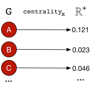
There exists numerous centrality measures that can be applied to a graph in order to rank its vertices according to how “centrally located” they are. Such measures are generally defined as:centralityx: G → ℝ+|V|
A centrality measure will map (→) a graph (G) to a positive real number vector/array (ℝ+) of size |V|. The resultant vector contains the “centrality” score for each vertex in the graph — Map<Vertex,Double>.
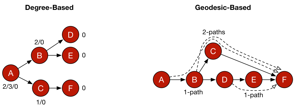
Five common centrality measures are presented in the table below. Along with each measure is the means by which the measure is calculated. Degree-based centralities are founded on the degree of a vertex and for PageRank and eigenvector centrality, in a recursive manner, on the degree of its adjacent vertices. Closeness and betweenness centrality are geodesic-based centralities which leverage shortest paths through a graph in their calculation and thus, are not based on vertex degree — though in many situations, recursively defined degrees and shortest paths can be and often are correlated. Finally, for each metric, the computational complexity is provided denoting the time cost of executing the measure against a graph, where |V| and |E| are the size of the graph’s vertex and edge sets, respectively.
| Centrality Measure | Topological Aspect | Computational Complexity |
| Degree Centrality | Degree-Based | 𝒪(|V|) |
| PageRank Centrality | Degree-Based | 𝒪(|V|+|E|) |
| Eigenvector Centrality | Degree-Based | 𝒪(|V|+|E|) |
| Closeness Centrality | Geodesic-Based | 𝒪(|V|*(|V|+|E|)) |
| Betweenness Centrality | Geodesic-Based | 𝒪(|V|3) |
Understanding the Complexity of Betweenness Centrality |
|---|
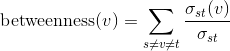
| The betweenness centrality of vertex v is defined as
where Conceptually, the simplest way to compute all shortest paths is to run Dijkstra’s algorithm from each vertex in the graph which, for any one vertex has a runtime of This callout box was written by Anthony Cozzie (DSEGraph Engineer).
|
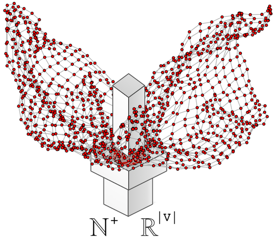
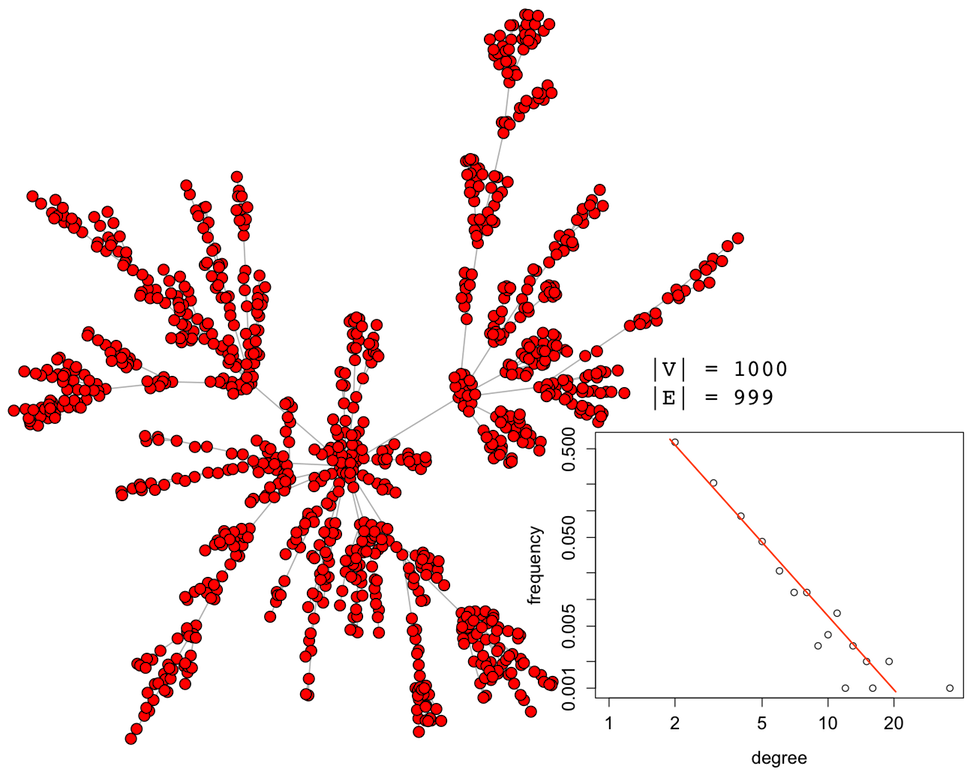
It should be apparent that geodesic-based centralities are more expensive than degree-based centralities. It is for this reason that in large-scale graph computations, it is important to avoid geodesics if possible. In other words, if another centrality measure yields the same or analogous rank vector but is cheaper to execute, then it should be leveraged in production. For instance, assume the following 1000 vertex scale-free graph generated using iGraph for the R:Statistics language.
g <- sample_pa(1000,directed=FALSE)plot(g, layout=layout.fruchterman.reingold, vertex.size=3, vertex.color="red", edge.arrow.size=0, vertex.label=NA) |
The five aforementioned centrality measures can be applied to this synthetically generated graph. Each centrality yields a vector with 1000 elements (i.e. |V|). Each of these vectors can be correlated with one another to create a correlation matrix. Given that the most important aspect of a centrality measure is the relative ordering of the vertices, the Spearman rank order correlation is used.
matrix <- cbind(centr_degree(g)$res,page.rank(g)$vector,eigen_centrality(g)$vector,closeness(g),betweenness(g))colnames(matrix) <- c("degree","pagerank","eigenvector","closeness","betweenness")cor(matrix,method="spearman") |
| Degree | PageRank | Eigenvector | Closeness | Betweenness | |
| Degree | 1.0000000 | 0.88429222 | 0.31932223 | 0.30950586 | 0.9927900 |
| PageRank | 0.8842922 | 1.00000000 | 0.05497317 | 0.04750024 | 0.8720052 |
| Eigenvector | 0.3193222 | 0.05497317 | 1.00000000 | 0.99336752 | 0.3218426 |
| Closeness | 0.3095059 | 0.04750024 | 0.99336752 | 1.00000000 | 0.3120138 |
| Betweenness | 0.9927900 | 0.87200520 | 0.32184261 | 0.31201375 | 1.0000000 |
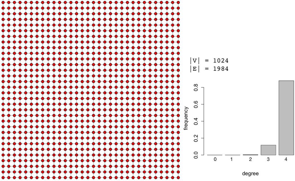
In the table above, for the specific synthetically generated scale-free graph, degree centrality and betweenness centrality are nearly perfectly correlated with ρ=0.9928. It would be prudent to use degree centrality instead of betweenness centrality as the computational complexity goes from 𝒪(|V|3) to 𝒪(|V|) and still yields a nearly identical rank vector. It is important to stress that this correlation matrix is specific to the presented graph and each graph instance will need to create it own correlation matrix. Thus, it isn’t always the case that degree and betweenness centrality are so strongly correlated. Identifying centrality correspondences must be determined on a case-by-case basis. As a counter example, a 1024 vertex 2-dimensional lattice graph has the following correlation matrix.
g <- make_lattice(length=32, dim=2)plot(g, layout=layout.grid, vertex.size=3, vertex.color="red", edge.arrow.size=0, vertex.label=NA)matrix <- cbind(centr_degree(g)$res,page.rank(g)$vector,eigen_centrality(g)$vector,closeness(g),betweenness(g))colnames(matrix) <- c("degree","pagerank","eigenvector","closeness","betweenness") cor(matrix,method="spearman") |
| Degree | PageRank | Eigenvector | Closeness | Betweenness | |
| Degree | 1.0000000 | 0.5652051 | 0.5451981 | 0.4773026 | 0.5652057 |
| PageRank | 0.5652051 | 1.00000000 | -0.3729564 | -0.4237888 | -0.3582003 |
| Eigenvector | 0.5451981 | -0.3729564 | 1.00000000 | 0.9890972 | 0.9960206 |
| Closeness | 0.4773026 | -0.4237888 | 0.9890972 | 1.00000000 | 0.9752467 |
| Betweenness | 0.5652057 | -0.3582003 | 0.9960206 | 0.9752467 | 1.0000000 |
In the above lattice graph correlation matrix, degree centrality and betweenness centrality have a ρ=0.565 which is a positive, though not a strongly correlated relationship. Furthermore, notice that in this particular lattice, the popular PageRank algorithm is negatively correlated with most of the other centrality measures. In this way, lattices do not offer a good alternative for the semantics of PageRank centrality.
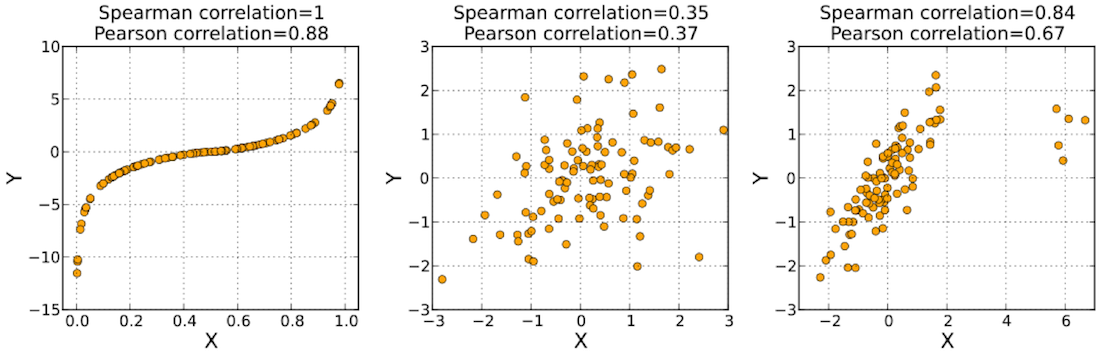
Understanding Correlation Methods |
|---|
|
|
Using Scale-Free Subgraphs for Centrality Correlations
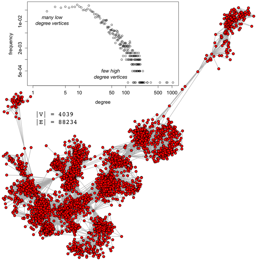
A Facebook social graph was derived via survey administered by Julian McAuley and Jure Leskovec and made publicly available on the Stanford SNAP archive. This real-world graph (i.e. not synthetically generated) is scale-free in that most vertices have few edges and few vertices have many edges. The graph’s correlation matrix for the 5 aforementioned centrality measures is provided below using the Spearman rank order correlation.
| Degree | PageRank | Eigenvector | Closeness | Betweenness | |
| Degree | 1.0000000 | 0.8459264 | 0.5270274 | 0.4300193 | 0.7881420 |
| PageRank | 0.8459264 | 1.00000000 | 0.2122095 | 0.2367609 | 0.7602193 |
| Eigenvector | 0.5270274 | 0.2122095 | 1.00000000 | 0.4484385 | 0.4133148 |
| Closeness | 0.4300193 | 0.2367609 | 0.4484385 | 1.00000000 | 0.4791568 |
| Betweenness | 0.7881420 | 0.7602193 | 0.4133148 | 0.4791568 | 1.0000000 |
Note that degree centrality and betweenness centrality are strongly correlated (ρ=0.788). Furthermore, degree centrality and PageRank centrality are strongly correlated (ρ=0.846). This means, that if Facebook were interested in determining the betweenness or PageRank centrality of their social graph, it would be much cheaper (computationally) to simply use degree centrality given the strength of the correlations between the respective measures.
In many real-world situations, graphs can be so large that to determine the above correlation matrix is expensive and furthermore, once the centrality measures are computed for correlation, it would be prudent to simply use the desired centrality measure’s result. However, one of the interesting aspects of scale-free graphs is that they are fractal in nature. This means that any connected subset of the full graph maintains the same (or similar) statistical properties. Much like the Mandelbrot set ![]() , it is possible to “zoom into” a scale-free graph and bear witness to yet another scale-free graph with analogous structural features.
, it is possible to “zoom into” a scale-free graph and bear witness to yet another scale-free graph with analogous structural features.
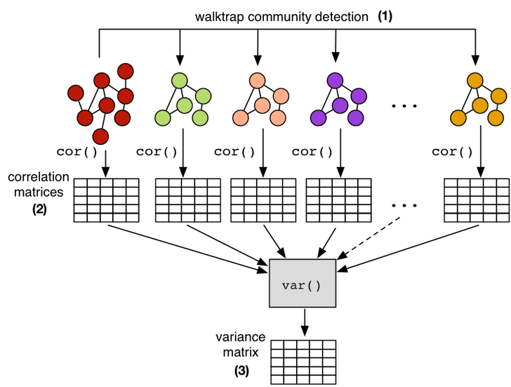
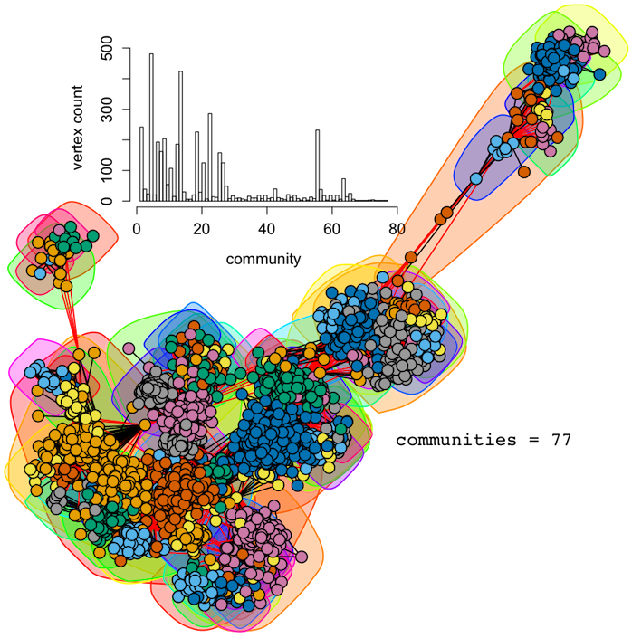
This self-similar aspect of scale-free graphs makes it possible to calculate a correlation matrix on a smaller subgraph of the larger graph and maintain confidence that the subgraph correlations will generalize to the full graph. Thus, for instance, instead of calculating the centrality correlation matrix on a 1 billion vertex graph, it is possible to calculate it on a 10,000 vertex subgraph, where the latter subgraph will be much easier to handle both in terms of time (computational complexity) and space (data set size). In order to demonstrate this point, the 10 largest communities in the presented Facebook graph are extracted using the random walk inspired walktrap community detection algorithm. Each subgraph community is then subjected to the 5 centrality measures in order to yield a respective correlation matrix. Finally, all 11 correlation matrices (full graph and 10 communities) are reduced to a single variance matrix which denotes the stability of the correlations across all matrices/subgraphs. This statistical workflow yields a result that is in accord with the theory of scale-free graphs as there is very little variance amongst the correlations across its fractal components.
# (1) isolate subgraphs using the walktrap community detection algorithmcommunities <- cluster_walktrap(g)membership <- membership(communities)histogram <- hist(membership,breaks=max(membership))sorted_communities <- sort(histogram$counts, decreasing=TRUE, index.return=TRUE)# (2) create correlation matrices for the 10 largest communitieslist <- list(cor(matrix,method="spearman"))for(i in sorted_communities$ix[1:10]) { subgraph <- induced_subgraph(g,communities[[i]],impl="create_from_scratch") submatrix <- cbind(centr_degree(subgraph)$res,page.rank(subgraph)$vector, eigen_centrality(subgraph)$vector,closeness(subgraph), betweenness(subgraph)) colnames(submatrix) <- c("degree","pagerank","eigenvector","closeness","betweenness") list <- append(list,list(cor(submatrix,method="spearman")))}# (3) reduce the correlation matrices to a single variance matrixapply(simplify2array(list),1:2, var) |
| Degree | PageRank | Eigenvector | Closeness | Betweenness | |
| Degree | 0.000000000 | 0.004386645 | 0.01923375 | 0.03285931 | 0.01544800 |
| PageRank | 0.004386645 | 0.000000000 | 0.06718792 | 0.06625113 | 0.00799879 |
| Eigenvector | 0.019233753 | 0.067187923 | 0.000000000 | 0.03008761 | 0.05339487 |
| Closeness | 0.032859313 | 0.066251132 | 0.03008761 | 0.000000000 | 0.03480015 |
| Betweenness | 0.015448004 | 0.007998790 | 0.05339487 | 0.03480015 | 0.000000000 |
Conclusion
The fields of graph theory and network science offer numerous statistical algorithms that can be used to project a complex graph structure into a smaller space in order to make salient some topological feature of the graph. The centrality measures presented in this article project a |V|2-space (i.e. an adjacency matrix) into a |V|-space (i.e. a centrality vector). All centrality measures share a similar conceptual theme — they all score the vertices in the graph according to how “central” they are relative to all other vertices. It is this unifying concept which can lead different algorithms to yield the same or similar results. Strong, positive correlations can be taken advantage of by the graph system architect, enabling them to choose a computationally less complex metric when possible.