ColBERT is a vector search algorithm that combines the signal from multiple vectors per passage to improve search relevance compared to single-vector retrieval. In particular, ColBERT largely solves the problems with out-of-domain search terms. My introduction to ColBERT gives a simple, pure Python implementation of ColBERT search.
But for production usage, the only option until now has been the Stanford ColBERT library and the Ragatouille wrapper. These are high performance libraries, but they only support use cases that can fit in a two-stage pipeline of (1) ingest all your data and then (2) search it. Updating indexed data is not supported, and integrating with other data your application cares about (such as ACLs) or even other parts of the indexed data (creation date, author, etc) is firmly in roll-your-own territory.
This post introduces the ColBERT Live! library for production-quality ColBERT search with an off-the-shelf vector database. This addresses both of the limitations of Stanford ColBERT:
- ColBERT Live! enables you to combine ColBERT search with other predicates or filters natively at the database level instead of trying to sync and combine multiple index sources in application code.
- ColBERT Live! supports realtime inserts and updates without rebuilding the index from scratch (assuming that this is supported by the underlying database, of course).
Background
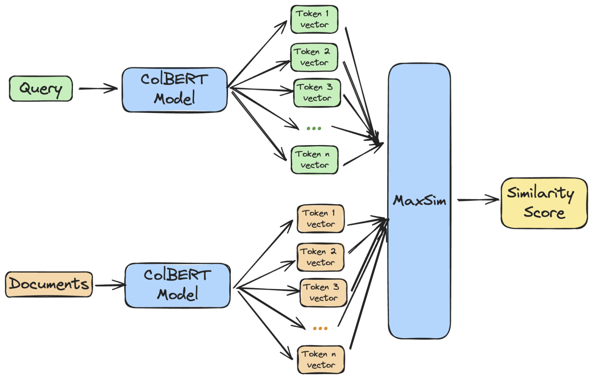
ColBERT breaks both queries and documents into vector-per-token, then computes the maximum similarity (maxsim) between each query vector and each document vector, and sums them together to arrive at the overall score. This gives more accurate results than hoping that your single-vector embedding model was able to capture the full semantics of your document in one shot.
 Image from Benjamin Clavié’s excellent article on ColBERT token pooling
There are thus three steps to a ColBERT search:
- Identify a subset of documents as candidates for maxsim computation
- Fetch all the embeddings for each candidate
- Compute the maxsim for each candidate
Since maxsim score computation is O(N x M) where N is the number of query vectors and M is the number of document vectors, ColBERT search is only feasible if we can restrict the candidate set somehow. In fact, each of these three steps can be optimized better than the brute force approach.
A stronger embeddings model
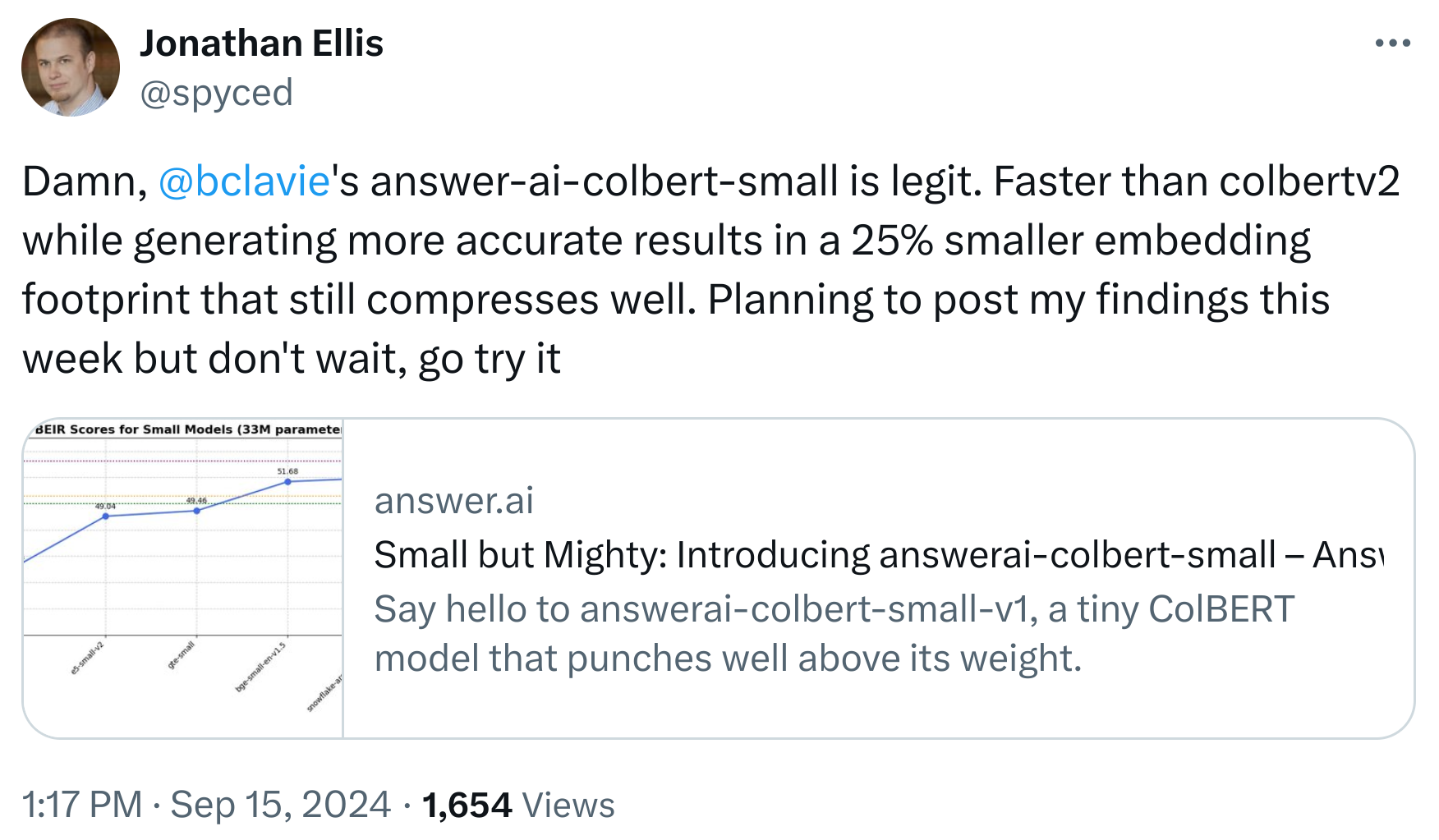
But first, let’s talk about how we generate embeddings in the first place. ColBERT Live! uses the Answer AI colbert-small-v1 model by default. Do read author Benjamin Clavié’s detailed explanation, but the summary is: this model is smaller (faster to compute embeddings), more aggressive at dimension reduction (faster searches), and better-trained (more relevant results) than the original.
Because all three stages of ColBERT search are O(N) in the embedding size, and colbert-small-v1 embeddings are 25% smaller than colbert-v2’s, we would expect to see about a 25% improvement in search times after switching from the colbert-v2 model to answerai-colbert-small-v1 and that is in fact what we observe.
Better candidate generation
In the original ColBERT research paper, and in my first article linked above, candidates are identified by performing standard single-vector searches for each of the query embeddings with the top k’ = k/2, then taking the union of those results.
The ColBERTv2 paper adds a custom index and a new candidate generation algorithm. The specifics are tightly coupled with the new index implementation, but the basic idea is simple enough:
- Fetch and score the document embeddings Dj that are nearest to each query vector Qi
- Group Dj by document, keeping only the best score from each document for each Qi
- Sum the scores for each document across all Qi
- Retrieve all embeddings from the top M documents for full maxsim scoring
Here is how this is implemented in colbert-live:
def search(self,
           query: str,
           n_ann_docs,
           n_maxsim_candidates
           ) -> List[Tuple[Any, float]]:
   """
   Q = self.encode_query(query)
   query_encodings = Q[0]

   # compute the max score for each term for each doc
   chunks_per_query = {}
   for n, rows in enumerate(self.db.query_ann(query_encodings, n_ann_docs)):
       for chunk_id, similarity in rows:
           key = (chunk_id, n)
           chunks_per_query[key] = max(chunks_per_query.get(key, -1), similarity)
   if not chunks_per_query:
       return []  # empty database

   # sum the partial scores and identify the top candidates
   chunks = {}
   for (chunk_id, qv), similarity in chunks_per_query.items():
       chunks[chunk_id] = chunks.get(chunk_id, 0) + similarity
   candidates = sorted(chunks, key=chunks.get, reverse=True)[:n_maxsim_candidates]

   # Load document encodings
   D_packed, D_lengths = self._load_data_and_construct_tensors(candidates)

   # Calculate full ColBERT scores
   scores = colbert_score_packed(Q, D_packed, D_lengths, config=self._cf)

   # Map the scores back to chunk IDs and sort
   results = sorted(zip(candidates, scores), key=lambda x: x[1], reverse=True)

   # Convert tensor scores to Python floats and return top k results
   return [(chunk_id, score.item()) for chunk_id, score in results[:k]]
This accelerates the search by a factor of about 3 for equal relevance.
A practical note: since relevance will suffer if the correct candidates aren’t found during the ANN query stage, it’s important to use a very high ANN top k (n_ann_docs). Fortunately, the performance impact of doing this is low compared to increasing the maxsim candidate pool size.
Document embedding pooling
ColBERT Live! supports document embedding pooling, which aims to eliminate low-signal vectors from the document embeddings. Author Benjamin Clavié has a full writeup here but the short version is that document embedding pooling reduces the number of vectors per document by approximately the pooling factor, i.e. a corpus indexed with pooling factor of 2 would have ½ as many vectors as an unpooled index, and with pooling factor of 3 ⅓ as many.
This means that less work has to be done in stages (2) and (3) of the search. In ColBERT Live!, a pool factor of 2 reduces search times by about 1/3. We’ll look at the tradeoff vs relevance below. (The details for ColBERT Live! are not quite the same as for Stanford ColBERT in Benjamin’s article.)
Query embedding pooling
Inspired by Benjamin’s work on document pooling, I implemented a similar approach for query embeddings. Compared to pooling document embeddings, I found that
- Clustering by cosine distance threshold works much better than clustering with a target number of clusters and euclidean distance
- Re-normalizing the pooled vectors is critical to preserving relevance
Here's the code:
def _pool_query_embeddings(query_embeddings: torch.Tensor, max_distance: float, use_gpu: bool) -> torch.Tensor:
   # Convert embeddings to numpy for clustering
   embeddings_np = query_embeddings.cpu().numpy()
   # Cluster
   clustering = AgglomerativeClustering(
       metric='cosine',
       linkage='average',
       distance_threshold=max_distance,
       n_clusters=None
   )
   labels = clustering.fit_predict(embeddings_np)

   # Pool the embeddings based on cluster assignments
   pooled_embeddings = []
   for label in set(labels):
       cluster_indices = np.where(labels == label)[0]
       cluster_embeddings = query_embeddings[cluster_indices]
       if len(cluster_embeddings) > 1:
           # average the embeddings in the cluster
           pooled_embedding = cluster_embeddings.mean(dim=0)
           if use_gpu:
               pooled_embedding = pooled_embedding.cuda()
           # re-normalize the pooled embedding
           pooled_embedding = pooled_embedding / torch.norm(pooled_embedding, p=2)
           pooled_embeddings.append(pooled_embedding)
       else:
           # only one embedding in the cluster, no need to do extra computation
           pooled_embeddings.append(cluster_embeddings[0])

   return torch.stack(pooled_embeddings)
Query embedding pooling reduces the number of query vectors and hence the work done in stages (1) and (3) of the search. Using a distance of 0.03 with the Answer AI model reduces search time by about 10%, while improving relevance on most BEIR datasets.
Combining document and query embedding pooling gives a compounded speedup, while improving the relevance problems that we see when using document embedding pooling alone.
Pooling effect on search relevance and speed
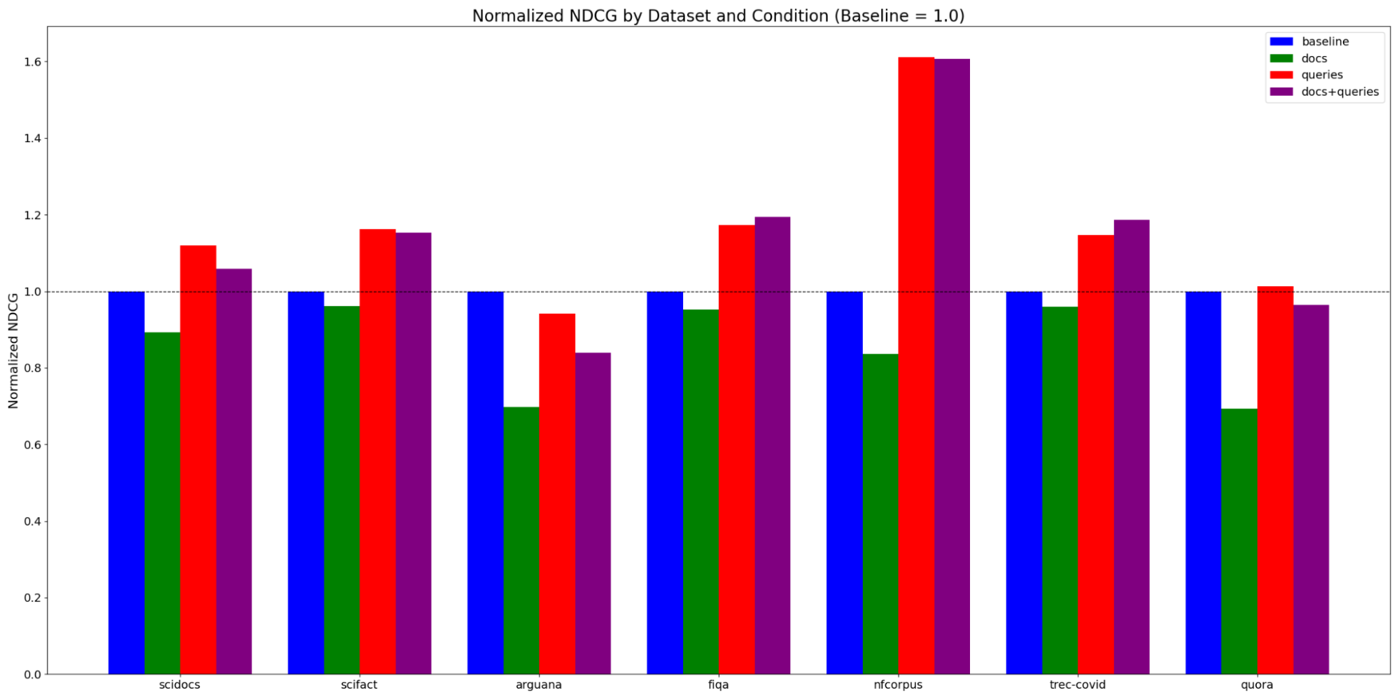
To visualize this, here’s a look at NDCG@10 scores for some of the BEIR datasets, normalized to the baseline score without pooling (at n_ann_docs=240, n_maxsim_candates=20). Query embedding pool distance is 0.03 (the default in ColBERT Live!, based on the histogram of distances between ColBERT embedding vectors), and document pooling clustering is 2.

Query embedding pooling is virtually a free lunch, improving relevance while also making searches faster. (The exception is arguana, which tests duplicate detection. Neither ColBERT nor ColBERT Live! optimizes for this use case.)
Document embedding pooling is more of a mixed bag, offering a significant speedup but also a significant hit to accuracy, although interestingly, adding query embedding pooling on top sometimes helps more than proportionally.
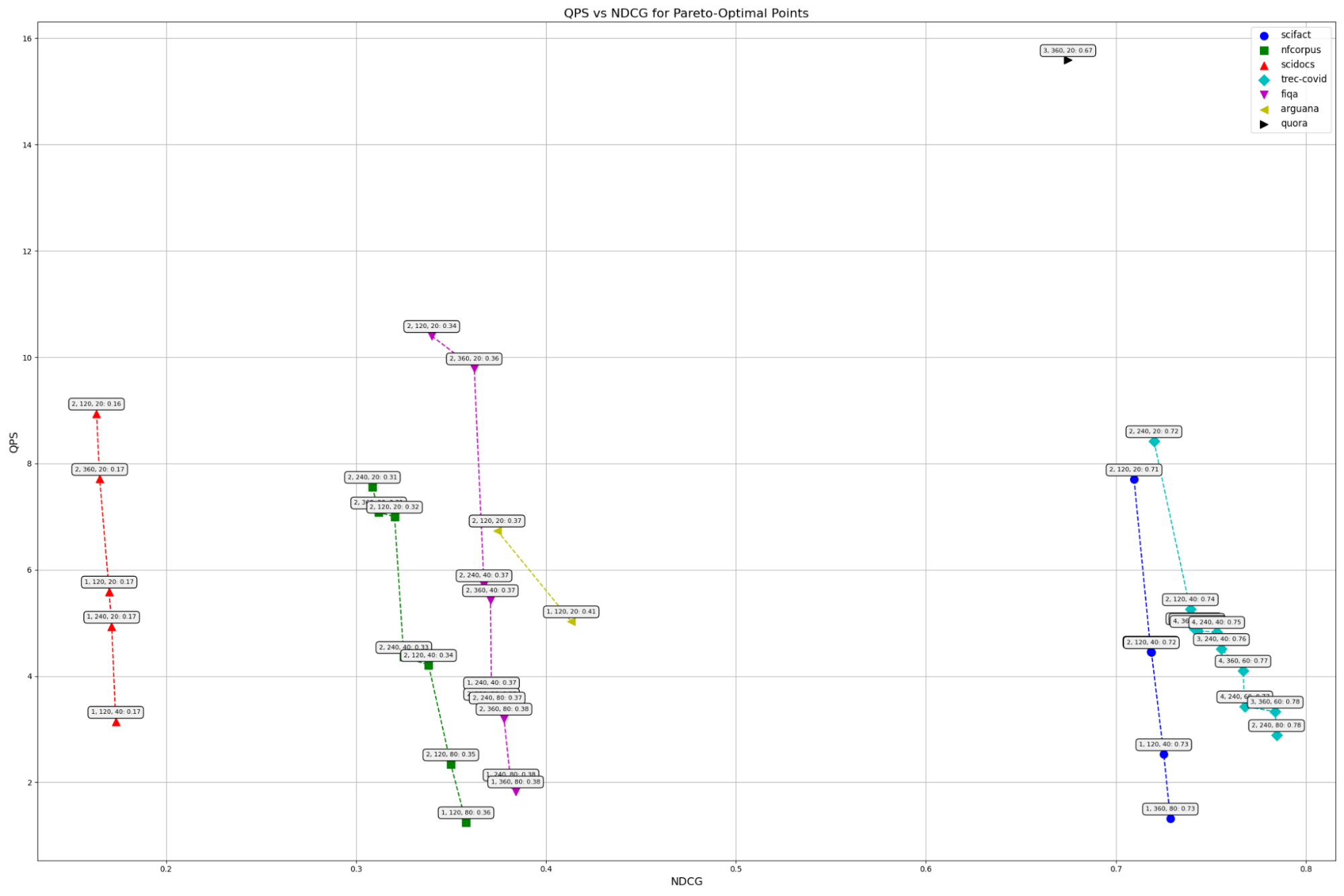
To see if the trade is worth it, let’s look at more data points. All of these use query embedding pooling distance of 0.03, but vary the other search parameters to see where the optimal tradeoff between speed and accuracy is. The X-axis is NDCG@10 score, and the Y axis is queries per second.
Points that are strictly worse in both QPS or NDCG for a given series are not shown. The point labels are doc pool factor, n_ann_docs, n_maxsim_candidates: ndcg@10, and the lines are color-coded by dataset. So the farthest point on the left of 2, 120, 20: 0.16 in red means that with doc_pool_factor=2, n_ann_docs=120, n_maxsim_candidates=20, we scored 0.16 on the scidocs dataset with about 9 QPS.
(There is only a single point shown for quora because all the other settings scored worse on both QPS and NDCG.)

My takeaways are:
- Document embedding pooling factor of 2 with query embedding pooling distance of 0.03 always achieves a reasonable place on speed:relevance, so that is what ColBERT Live! defaults to.
- You can increase relevance from that starting point but the cost is significant. Usually, you have to increase n_maxsim_candidates to do so.
- If you do need the extra relevance, increasing
n_maxsim_candidatesis a better way to do that than eliminating document embedding pooling. - However, increasing document embedding pooling more than 2 is often a bad trade
Using ColBERT Live!
If you look at the code sample under “better candidate generation”, you will see that there are two methods that must be implemented by the user:
db.query_ann, to perform a search for a single query vectordb.query_chunks, to load all the embeddings associated with a given document (called by_load_data_and_construct_tensors)
In fact these are the only two methods that need to be implemented. You can do this at the lowest level by implementing the DB abstract class, or you can subclass a vendor-specific class like AstraDB that given you convenient tools for schema management and parallel querying.
The ColBERT Live! Repo includes a full example of creating a simple command-line tool to add and search documents to an Astra database.
When to use ColBERT Live!
ColBERT Live! Incorporates the latest techniques from Stanford ColBERT and Answer.AI and introduces new ones to reduce the overhead of combining multiple vectors while maintaining high query relevance.
Consider using ColBERT Live! if you need a robust, production-ready semantic search that offers state-of-the-art performance with out-of-domain search terms that can also integrate with your existing vector database.
Get it from pypi (pip install colbert-live) or check it out on github!


