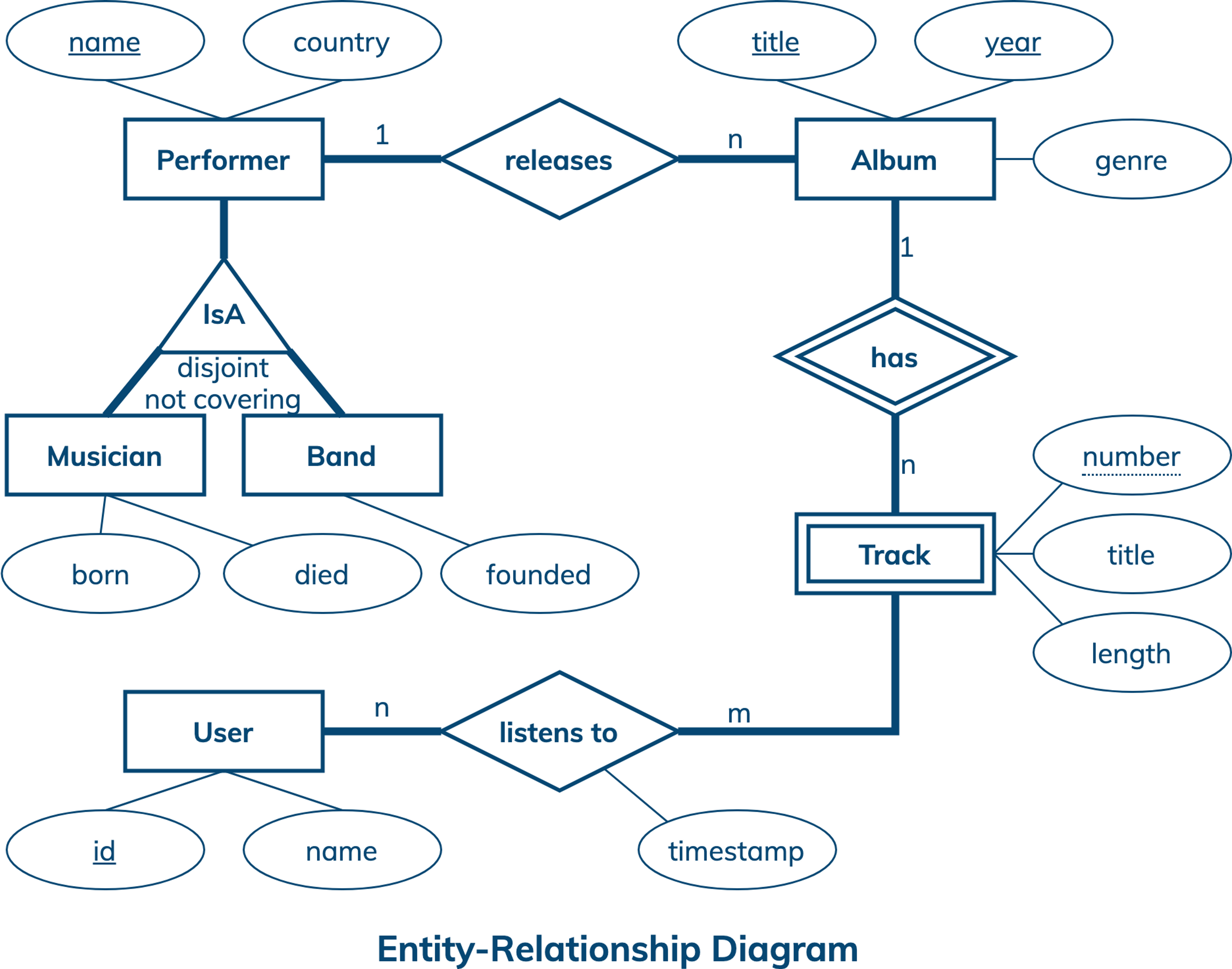
A conceptual data model is designed with the goal of understanding data in a particular domain. In this example, the model is captured using an Entity-Relationship Diagram (ERD) that documents entity types, relationship types, attribute types, and cardinality and key constraints.

The conceptual data model for the digital music library features performers, albums, album tracks and users. A performer has a unique name and is usually classified as a musician or a band. While any performer can have a country affiliation, only a musician can have born and died years and only a band can have a year of when it was founded. An album is uniquely identified by its title and release year, and also features genre information. A track has a number, title and length, and is uniquely identified by a combination of an album title, album year and track number. A user has a unique id and may have other attributes like name. While a performer can release many albums, each album can only belong to one performer. Similarly, an album can have many tracks, but a track always belongs to exactly one album. Finally, a user can listen to many tracks and each track can be played by many users.

An application workflow is designed with the goal of understanding data access patterns for a data-driven application. Its visual representation consists of application tasks, dependencies among tasks, and data access patterns. Ideally, each data access pattern should specify what attributes to search for, search on, order by, or do aggregation on.

The application workflow diagram has five tasks and nine data access patterns. Four out of five tasks are entry-point tasks. In addition, there can be many different paths in this workflow to explore. One possible scenario is described as follows. First, an application shows a user information and her recent music listening history by retrieving data using data access patterns Q8 and Q9. Second, the user searches for a performer with a specific name, which is supported by Q1. Third, the next task retrieves all albums of the found performer using Q2. The resulting list of albums should be sorted using release years, showing the most recent albums first. Finally, the user picks an album and the application retrieves all the album tracks sorted in the ascending order of their track numbers, which requires data access pattern Q7. At this point, the user may decide to listen to a specific track or the whole album, which would be reflected in her listening history. Alternatively, the user may go back to the album selection task or start a new path by looking for performers, albums or tracks. Take a look at the remaining data access patterns and additional paths in this workflow.

A logical data model results from a conceptual data model by organizing data into Cassandra-specific data structures based on data access patterns identified by an application workflow. Logical data models can be conveniently captured and visualized using Chebotko Diagrams that can feature tables, materialized views, indexes and so forth

The logical data model for digital library data is represented by the shown Chebotko Diagram. There are eight tables that are designed to support nine data access patterns. Table performers has single-row partitions with column name being a partition key. This table can efficiently satisfy Q1 by retrieving one partition with one row. Tables albums_by_performer, albums_by_title and albums_by_genre have multi-row partitions. While these tables store the same data about albums, they organize it differently and support different data access patterns. Table albums_by_performer stores one partition per performer with rows representing albums, such that all albums released by a specific performer can be always retrieved from a single partition using Q2. Table albums_by_title supports two data access patterns Q3 and Q4 to retrieve albums based on only album title or both title and year. Q3 may return multiple rows and Q4 may return at most one row. Both Q3 and Q4 only access one partition. Table albums_by_genre is designed to support Q5 that retrieves all albums from a known genre in the descending order of their release years. Next, tables tracks_by_title and tracks_by_album are designed to efficiently support data access patterns Q6 and Q7, respectively. Given a track title, Q6 can retrieve all matching tracks and their information from a single partition of table tracks_by_title. Given an album title and year, Q7 can retrieve all album tracks from a single partition of table tracks_by_album. In case of Q7, returned album tracks are always ordered in the ascending order of track numbers, which is directly supported by the table clustering order. Also, notice that column genre in table tracks_by_album is a static column whose value is shared by all rows in the same partition. This works because genre is an album descriptor and the partition key in this table uniquely identifies an album. Finally, tables users and tracks_by_user are designed to support Q8 and Q9. While the former has single-row partitions and the latter has multi-row partitions, partitions from both tables can be retrieved based on user ids.

A physical data model is directly derived from a logical data model by analyzing and optimizing for performance. The most common type of analysis is identifying potentially large partitions. Some common optimization techniques include splitting and merging partitions, data indexing, data aggregation and concurrent data access optimizations.

The physical data model for digital library data is visualized using the Chebotko Diagram. This time, all table columns have associated data types. In addition, table tracks_by_user has a new column as part of its partition key. The optimization here is to split potentially large partitions by introducing column month, which represents the first day of a month, as a partition key column. Consider that a user who plays music non-stop generates a new row for table tracks_by_user every 3 minutes, where 3 minutes is an average track length estimate. The old design allows partitions to grow over time: 20 rows in an hour, 480 rows in a day, 3360 rows in a week, 13440 rows in 4 weeks, 175200 rows in a non-leap year, and so forth. The new design restricts each partition to only contain at most 14880 rows that can be generated in a month. Our final blueprint is ready to be instantiated in Cassandra.