KNN identifies the K-nearest neighbors to a given data point using a distance metric, making predictions based on similar data points in the dataset. It is also useful in benchmarking Approximate Nearest Neighbors (ANN) search indexes. ANN searches are the most commonly used vector search technique as they are (many) orders of magnitude faster than brute-force KNN searches against high-dimensional data–but this speed comes at the cost of retrieval accuracy. KNN can be used to measure this loss of accuracy, allowing ANN parameters to be adjusted to strike an appropriate balance of accuracy and speed.
This guide will delve into the fundamentals of the KNN algorithm, its workings, and its applications, grounded in the context of vector search.
An introduction to K-Nearest Neighbors (KNN) algorithm
The KNN algorithm operates on the principle of similarity or “nearness,” predicting the label or value of a new data point by considering the labels or values of its K-nearest (the value of K is simply an integer) neighbors in the training dataset.
Consider the following diagram:
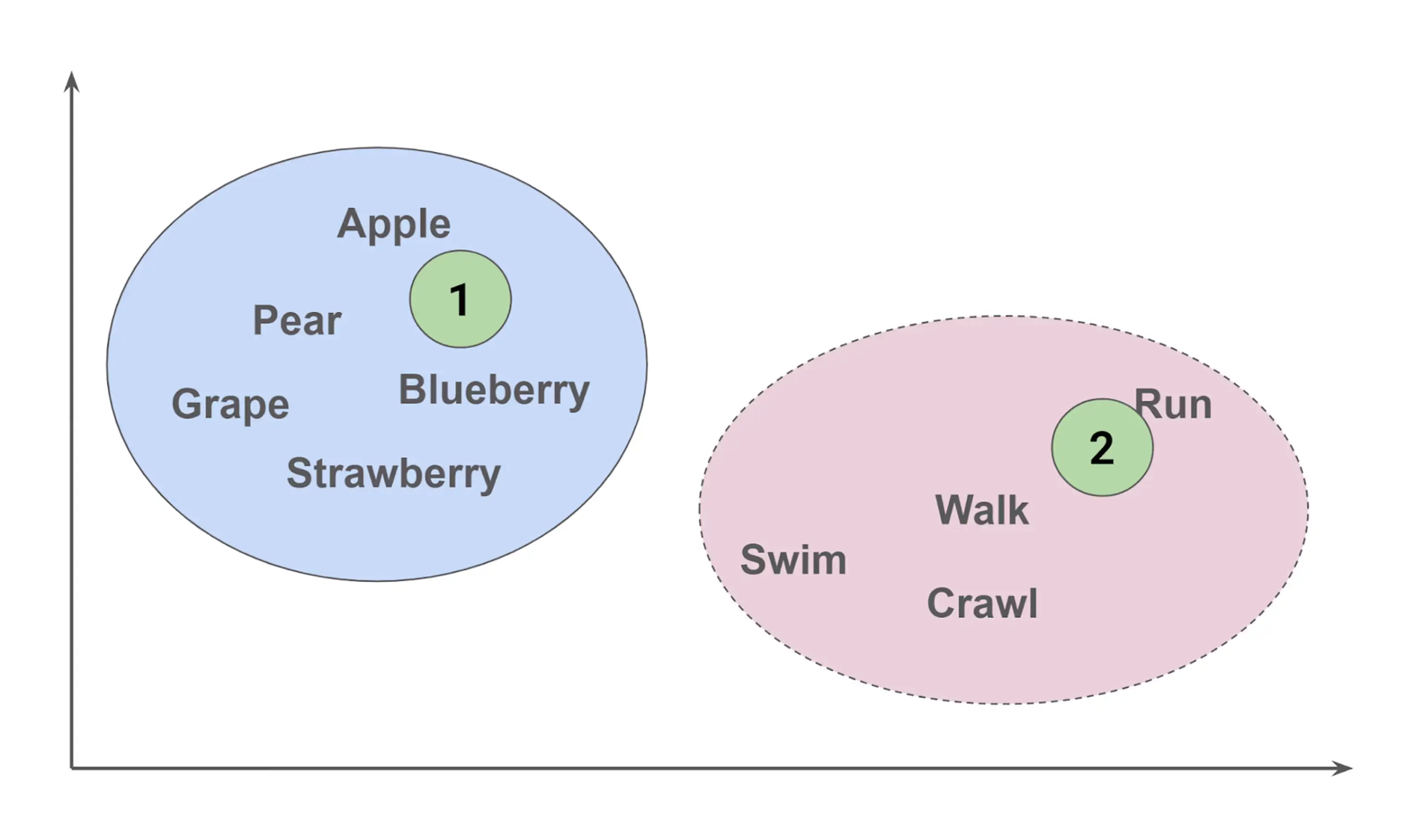
In the solid blue oval are kinds of fruit (nouns), and in the dashed pink oval are kinds of actions (verbs). So if we had a new word in position 1 in the solid blue oval, we would probably categorize it as a “fruit.” If we had to guess what the word in position 2 in the dashed pink oval was, humans might come up with a word like “jog” – but the KNN algorithm would pick “run” as the word because “jog” is not in its vocabulary, and point 2 is nearest to “run.”
In addition to categorizing and predicting new words, KNN can also perform numeric regression. For instance, if actions in the dashed pink oval have associated speeds, the algorithm can predict the speed for a new action at position 2 by averaging the speeds of its nearest neighbors.
This is an example of KNN: based on the relative position of a new value to existing values, we can determine the category a new value belongs to (as in the word 1 example), predict a value for a new word (as in the word 2 example), and perform numeric regression by combining the values of the nearest neighbors.
Key features of the KNN algorithm
- Simplicity and Ease of Implementation: KNN is straightforward to implement and understand, making it one of the first algorithms introduced to data science beginners.
- Instance-Based and Lazy Learning Characteristics: Unlike many other algorithms, KNN does not build a model during the training phase. Instead, it memorizes the training dataset and performs computations only when making predictions.
- Non-Parametric Nature: KNN makes no assumptions about the underlying data distribution, which allows it to be applied to various types of data.
- Fast Training Time: KNN’s training phase is very fast - it only involves storing the data!
- Slow Prediction Time: Inversely, KNN’s prediction speed is slow: brute-force search is on the order of data points times dimensionality.
- Data Point Based: The KNN algorithm predicts outcomes by analyzing the proximity of individual data points within a dataset, relying on data point relationships for accurate predictions.
Real-world applications of KNN
KNN is widely used within machine learning but it is also used as a tool for optimizing ANN searches.
Machine learning applications
As a vector search algorithm, KNN has many of the same applications as ANN search, but KNN can provide a guarantee of “closest matches” (at the expense of speed). Because it is easy to implement, KNN can be used as a “proof of concept” to build a more complex application such as neural networks, decision trees, and support vector machines.
Classification
- Spam Detection: KNN can classify emails as spam or not spam based on the similarity of their content to known spam and non-spam emails.
- Medical Diagnosis: By analyzing patient symptoms and medical history, KNN can assist in diagnosing diseases based on similar cases.
Regression
- Price Prediction: KNN can predict the price of a house or a stock based on historical data and features like location, size, and market trends.
Recommendation Systems
- Movie Recommendations: Streaming services leverage KNN to recommend movies based on a user's viewing history and similar users' preferences.
- Product Recommendations: E-commerce platforms utilize KNN to suggest products based on a user's browsing and purchase history.
Pattern Recognition
- Handwriting Recognition: Employ KNN to recognize handwritten characters by comparing them to a database of known characters.
Image Recognition
- Object Detection: KNN can identify objects in images based on their visual similarity to labeled objects in a training set.
Anomaly Detection
- Fraud Detection: By analyzing spending patterns and transaction history, KNN can flag potentially fraudulent activities based on deviations from normal behavior.
Measuring ANN performance
Most ANN algorithms have tunable parameters that can optimize the algorithm. For example, within the Hierarchical Navigable Small Worlds (HNSW) algorithm there are parameters to manage the number of layers, the density of each layer, and the number of connections between and within layers.
These parameters influence the speed and space requirements of the ANN index, but generally, the faster and smaller these indexes are, the more likely they are to miss the nearest neighbors. This is measured with something called “recall,” where 100% recall means all of the nearest neighbors are found. KNN always has a 100% recall!
To measure ANN recall performance, choose the same definition of how to measure “nearest” with a set of test data and learn how many of the true nearest neighbors (via KNN) have been missed by the ANN algorithm.
We do not generally care too much about KNN's slower performance in this context—we are treating it as a baseline reference. Further, we measure the K-nearest neighbors on any dataset once so we can adjust ANN parameters and quickly re-run the ANN evaluations.
How does the KNN algorithm work?
Break down the KNN algorithm's workflow into the following steps:
- Selecting the Value of K: Choose the number of nearest neighbors to consider.
- Calculating Distance: Compute the distance between the target data point and all points in the training data using a distance metric (discussed next).
- Finding Nearest Neighbors: Identify the K data points with the smallest distances to the target point.
- Prediction: For classification tasks, assign the class label based on the majority vote among the K neighbors. For regression tasks, take the average (or some other numeric combination) of the target values of the K nearest neighbors.
Computing KNN distance metrics
To find “nearest neighbor,” we need to have some way of defining “nearest”; for this we use a distance metric. Because we need to compare distances between a given point and all points in the dataset, KNN typically employs fast, low-complexity distance measures. Here are some commonly used measures:
- Euclidean Distance: The straight-line distance between two points in Euclidean space by taking the square root of the sum of the squared differences of their corresponding coordinates.
- Manhattan Distance: The distance between two points in a grid-based system by summing the absolute differences of their corresponding coordinates.
- Minkowski Distance: The distance between two points by combining aspects of both Euclidean and Manhattan distances, depending on an adjusted parameter.
- Cosine Similarity: Measures how similar two points are by calculating the cosine of the angle between their vectors, indicating how closely they point in the same direction.
The computational effort for Minkowski distance lies between that of Manhattan distance (easiest) and Euclidean distance (more effort), and the effort for Cosine similarity is generally greater than that for Euclidean distance.
In the following formulas, we will use the following notation:
| Formula Notations | |
|---|---|
| D | Distance between two points |
| pi | The value of the i-th dimension of some point p |
| s | The source point for the distance calculation |
| x | One of the training points for the distance calculation |
| d | The number of dimensions in the space |
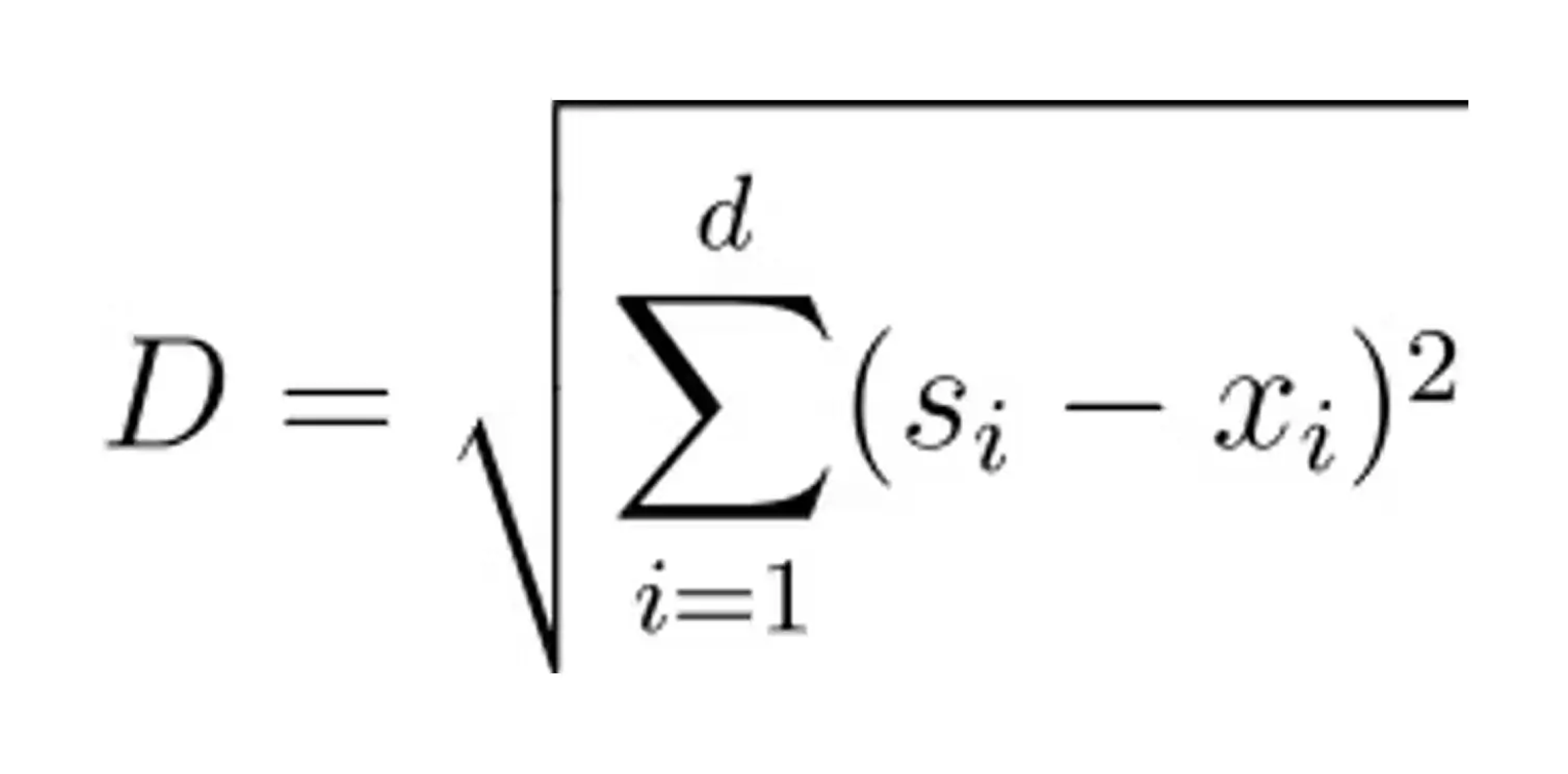
Euclidean Distance
Euclidean distance, often considered the most intuitive metric, calculates the straight-line distance between two data points in a multi-dimensional space. Its formula, rooted in the Pythagorean theorem, is straightforward:
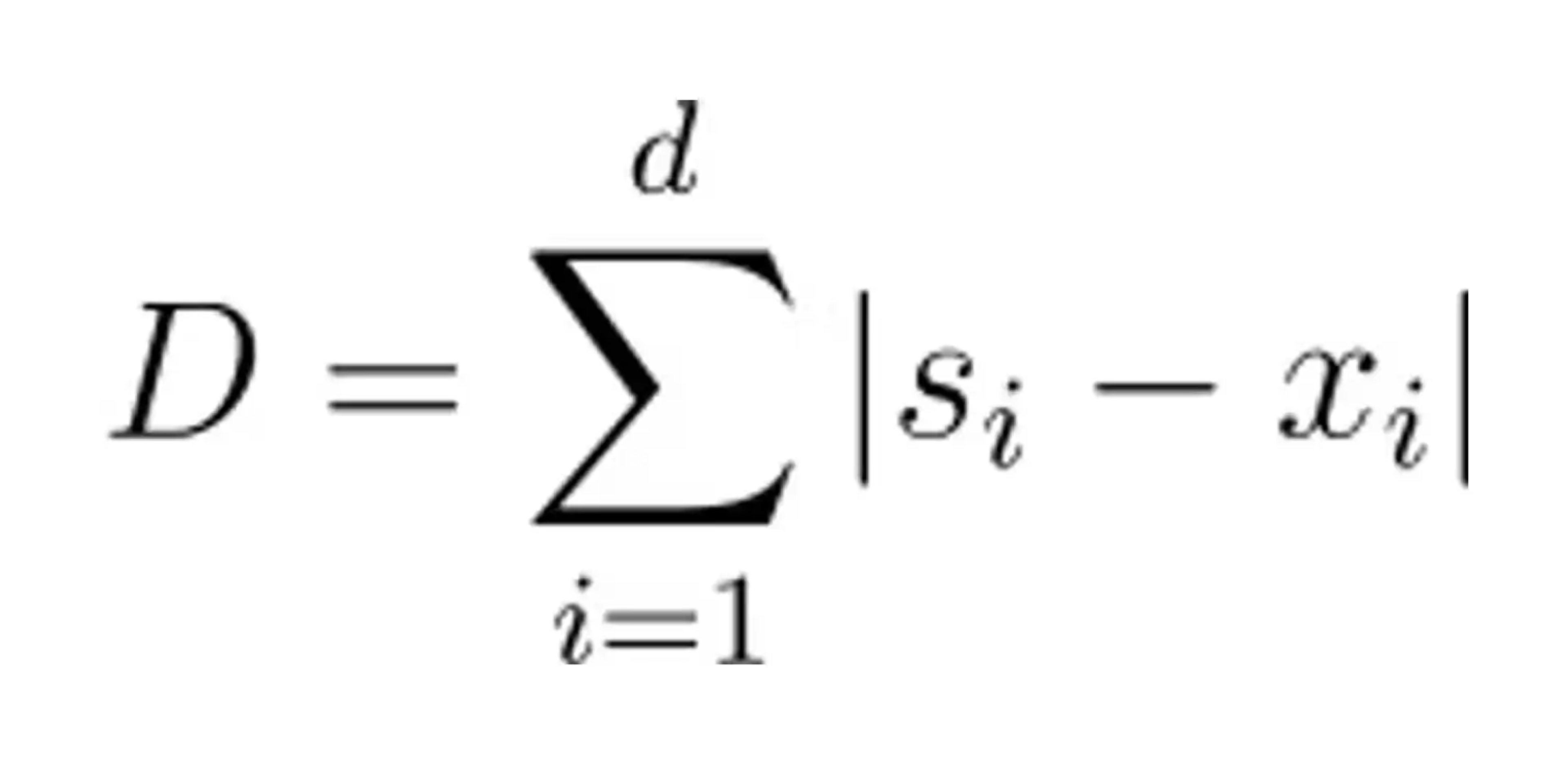
Manhattan Distance
Manhattan distance, also known as taxicab distance, measures the distance between two points by summing the absolute differences of their coordinates along each dimension. In two dimensions, visualize it as navigating a grid-like city block - you can only move horizontally or vertically.
Manhattan distances become particularly useful in sparsely-populated high-dimensional spaces as described by Aggarwal et al. (“On the Surprising Behavior of Distance Metrics in High Dimensional Spaces,” 2001), or if features have significantly different scales where a squaring of differences would tend to amplify the distances caused by larger numbers (imagine a feature with values between 0 and 10, compared to one that has values between 0 and 1).
The formula for Manhattan distance is as follows:
Minkowski Distance
Minkowski distance serves as a generalization of both Euclidean and Manhattan distances. It introduces a parameter p, a value between 1 and 2 that dictates the nature of the distance calculation. The formula for Minkowski distance is given by:
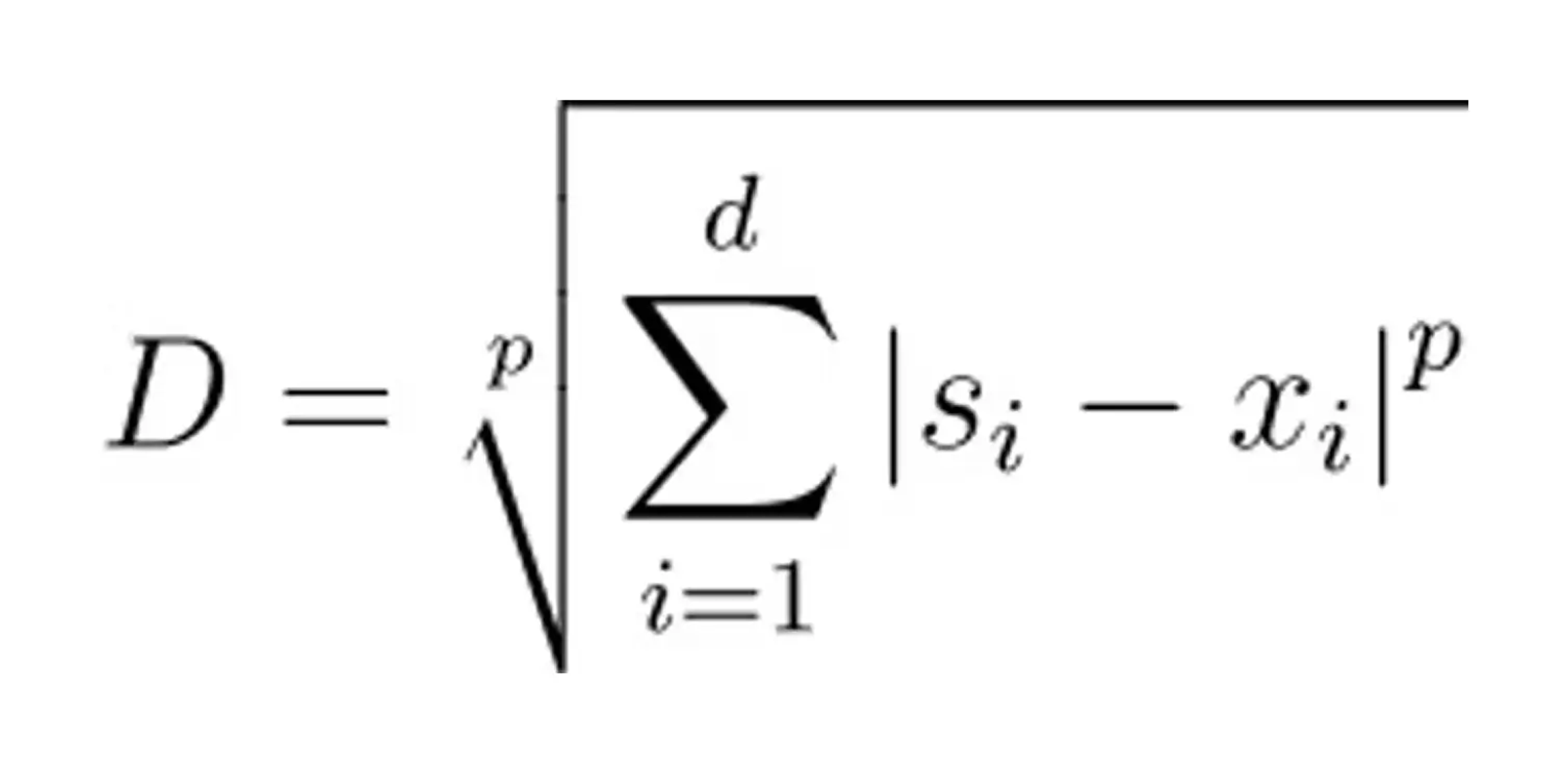
When p is set to 1, the Minkowski distance is equivalent to the Manhattan distance, and when p is set to 2, it is equivalent to the Euclidean distance.
Cosine Similarity
Cosine similarity measures the cosine of the angle between two vectors in a multi-dimensional space, indicating how similar the vectors are in terms of their direction. Unlike other distance metrics, cosine similarity focuses on the orientation rather than the magnitude, making it particularly useful in text analysis and high-dimensional data. The formula for cosine similarity is:
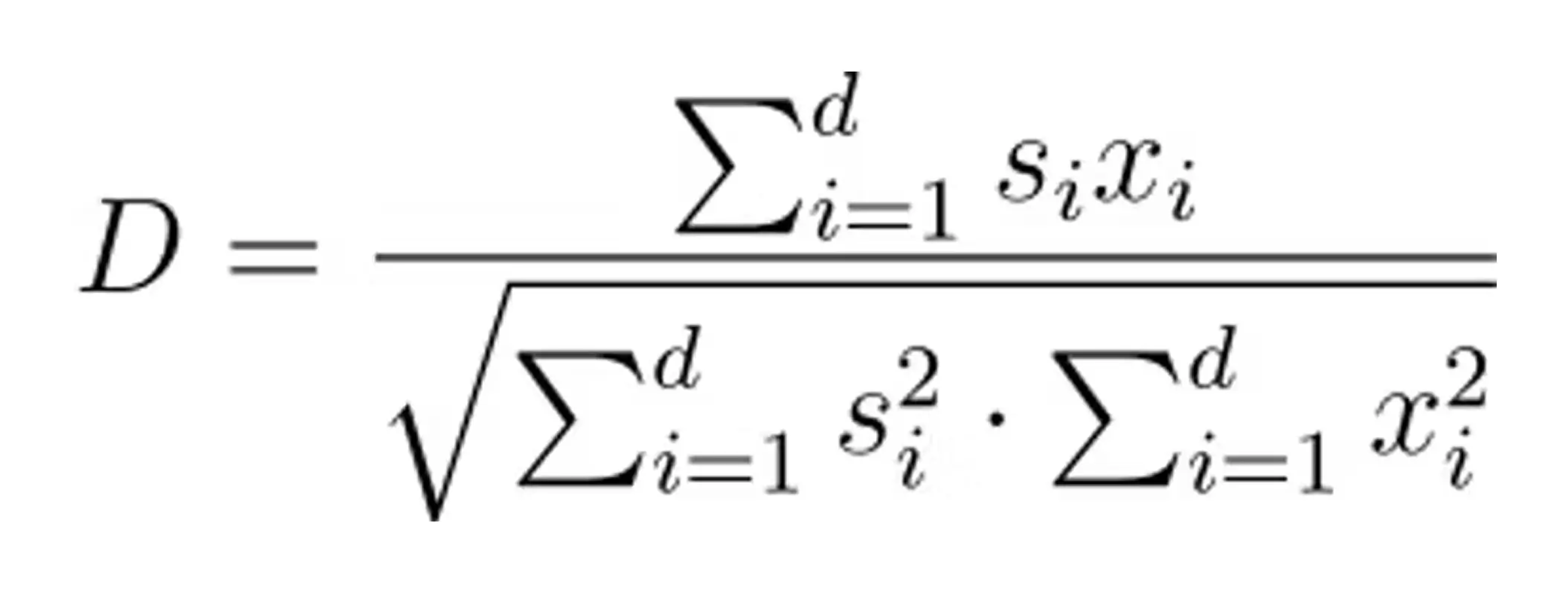
If the space is “normalized” (all vectors have a unit length of 1), only the numerator (dot product) needs to be computed. For a deeper explanation of cosine similarity, here’s an overview of cosine similarity or some other real-world use cases of cosine similarity, along with a deeper dive into the math.
Choosing the right vector top K value
Determining how many neighbors to find the top K value is application-dependent. If using KNN to validate ANN performance, the K value is generally the same as the ANN search K value, which is itself application-dependent!
In general, a small K value can lead to results that are overly sensitive to noise in the data, while a large K value may fail to capture the most relevant neighbors.
Several techniques can help determine the optimal K value for vector search applications, including:
- Cross-Validation: In this context, cross-validation involves partitioning the dataset into multiple subsets. The search algorithm's performance is evaluated on these subsets to determine the top K value that balances precision and recall.
- Elbow Method: This method plots the search error rate or a relevant performance metric against various K values. The 'elbow point' on the graph, where the improvement rate starts to slow down, often indicates a good choice for K. This point represents a balance between having too few and too many neighbors.
- Silhouette Analysis: Silhouette analysis measures how similar a point is to its own cluster (based on nearest neighbors) compared to other clusters. The silhouette coefficient ranges from -1 to 1, with higher values indicating better-defined clusters. By calculating the silhouette coefficient for various K values, one can choose the top K that maximizes this coefficient, thus ensuring optimal cluster separation and compactness.
- Grid Search: Grid search systematically works through multiple combinations of parameter values, in this case, different K values, to find the optimal parameter setting. This technique is computationally intensive but can be very effective. The best performing value can be selected by evaluating the performance of the search algorithm across a range of K values.
Employing these techniques can identify the top K value that optimally balances search accuracy and computational efficiency, thereby improving the vector search's performance and robustness.

Benefits and limitations of KNN
The KNN algorithm, like any other tool, comes with its own set of advantages and drawbacks:
Benefits
- Easy to Understand and Implement: KNN's intuitive nature makes it accessible to a wide range of users, from beginners to experienced practitioners.
- Adaptability to New Data: KNN can easily incorporate new data points without retraining the entire model.
- Versatility in Handling Different Data Types: KNN accommodates various data types, making it suitable for a broad spectrum of applications.
Limitations
- Computationally Expensive: Calculating distances between all data points, especially in large datasets, can be computationally intensive, impacting speed.
- Sensitivity to Outliers: KNN's performance can be significantly affected by outliers in the data.
- Sensitive to Irrelevant Features: Requires careful feature selection and scaling.
Vector search: KNN or ANN?
At first glance, it would seem that knowing the “exact” neighbors is preferable to only knowing the “approximate” neighbors. But for how long do you want to wait to find these? Most vector search applications have a user waiting (patiently) on the other end for the result – and in RAG-type applications, these results must first be sent to a large language model (LLM) before being sent to a user.
Imagine a vector database with 1 million documents, each with 768 dimensions in a normalized vector space. We would use cosine similarity to compare the distance, and really we can take the dot-product shortcut because the data is normalized.
To conduct a KNN search of one vector via “brute force,” we would need to compute 768 x 106 multiplications plus 767 x 106 additions (for the distance measurement), plus another 106 comparison operations, for a total of 1.536 x 10⁹ (billion) operations. Though this could certainly be done in a highly parallel fashion, that is a lot of calculations! Beygetzimer et al. demonstrated a cover tree index structure (“Cover trees for nearest neighbor”, 2006) that shows speedups of up to several orders of magnitude, though these are not widely used.
As an alternative approach, consider a widely-used ANN algorithm such as HNSW which typically needs to search O(log N) data points for high recall rates; In this case that will be about 20 (of the 1 million) points we need to compare to. This math works out to (768 + 767) x 20 + 20 = 30,720 operations: a factor of 50 million fewer comparisons!
ANN can often be tuned to achieve high 90s percent recall without dramatically increasing computational complexity. Indexing techniques such as jVector can further improve latency and space requirements of ANN indexes.
While some vector search applications may “need” a guarantee of 100% recall accuracy, in practice the vector embedding algorithms and LLM training limitations end up being the constraining factor in application accuracy and general performance.
Vector search built for real-world generative AI with DataStax
This guide explores the K-Nearest Neighbors (KNN) algorithm, highlighting its simplicity and versatility in handling classification and regression tasks. KNN is often a good starting point for building a machine learning application, but for most generative AI vector search applications it is often too slow, owing to the intensity of the computations. KNN is useful in evaluating and optimizing ANN search parameters, facilitating a testable assertion of ANN recall performance.
One example of such evaluation is found in an open-source tool called Neighborhood Watch. It has been built by DataStax engineering teams to create ground truth datasets for high-dimension embeddings vectors that are more representative of what people are actually using today. One aspect of the tool is the generation of KNN results using a brute-force approach, which leverages GPU acceleration to compute these results efficiently. The KNN results can then be tested against various ANN configurations, enabling the tuning and optimization of recall and precision metrics for specific use cases. The blog post Vector Search for Production: A GPU-Powered KNN Ground Truth Dataset Generator gives a more detailed overview of this.Such a real-world analysis of ANN recall performance using a KNN ground truth baseline has led DataStax to introduce a source_model parameter on vector indexes: testing found that recall and latencies are improved by adjusting some ANN parameters that vary depending on the embedding model.

KNN: Fine-tune vector search
The K-Nearest Neighbors (KNN) algorithm is a simple, powerful approach to vector search and machine learning tasks. It's easy to implement, and its versatility makes it valuable for proof-of-concept applications and benchmarking Approximate Nearest Neighbors (ANN) search performance.
KNN's shortfall is its computational intensity. It doesn't scale well for large datasets and real-time applications. While KNN guarantees 100% recall accuracy, modern vector search solutions often favor ANN algorithms for their superior speed and efficiency.
When properly tuned, the Approximate Nearest Neighbor algorithm achieves high recall rates with significantly reduced computational overhead. For most generative AI and vector search applications, ANN algorithms strike an optimal balance between accuracy and performance, making them the preferred choice in production environments.
KNN remains essential for evaluating and optimizing ANN search parameters to fine-tune vector search implementations for specific use cases.

%20Algorithm%3F%20%7C%20DataStax&_biz_n=0&rnd=491115&cdn_o=a&_biz_z=1744919412859)
%20Algorithm%3F%20%7C%20DataStax&_biz_n=1&rnd=72930&cdn_o=a&_biz_z=1744919412860)
%20Algorithm%3F%20%7C%20DataStax&rnd=982085&cdn_o=a&_biz_z=1744919412863)
