Gremlin Recipes: 10 – Depth-First Vs Breadth-First

Part 10 of 10 for the series Gremlin Recipes. The purpose is to explain the internal of Gremlin and give people a deeper insight into the query language to master it.

This blog post is the 9th from the series Gremlin Recipes. It is recommended to read the previous blog posts first:

1. Gremlin as a Stream
2. SQL to Gremlin
3. Recommendation Engine traversal
4. Recursive traversals
5. Path object
6. Projection and selection
7. Variable handling
8. sack() operator
9. Pattern Matching
    

I KillrVideo dataset

To illustrate this series of recipes, you need first to create the schema for KillrVideo and import the data. See here for more details.

The graph schema of this dataset is :

II Evaluation strategy in Gremlin

Familiar users of Gremlin know that there exist 2 distinct evaluation strategies for traversals:

1. depth-first: this strategy traverses down the entire path as specified by a the steps before turning to the next legal path. In theory there is a single traverser that explores each path but in practice for optimisation purposes, the vendors can implement concurrent traversers for distinct paths. The depth-first strategy is the default strategy in Gremlin unless specified otherwise.
2. breadth-first: this strategy tries to parallelize the traversal of each step as much as possible. On each step, Gremlin will explore all possible paths before moving to the next step in the traversal

Let’s take a the recommendation engine traversal we have seen in previous posts:

gremlin>g.V().
   has("movie", "title", "Blade Runner").                       // stage 1
   inE("rated").filter(values("rating").is(gte(8.203))).outV(). // stage 2
   outE("rated").filter(values("rating").is(gte(8.203))).inV()  // stage 3

The above traversal can be decomposed into 3 stages

1. has("movie", "title", "Blade Runner")
2. inE("rated").filter(values("rating").is(gte(8.203))).outV()
3. outE("rated").filter(values("rating").is(gte(8.203))).inV()

Below is how a concurrent depth-first strategy would work

From the Blade Runner movie vertex, some traversers start exploring down the traversal by navigating to user vertices and then to other movie vertices. Note each possible path can be explored in parallel by a traverser and at any time, each traverser can be at different stage with regard to the global traversal.

The same traversal using breadth-first strategy:

With this strategy there are as many traversers as there are legal paths in each stage. And the traversers move to the next stage only when all paths of the current stage have been explored.

III OLTP vs OLAP mode

Very closely related to the evaluation strategies is the Gremlin execution mode: OLTP or OLAP. The below table gives a summary of the characteristics of each execution mode:

By default, Gremlin uses the OLTP execution mode which interacts with a limited set of data and respond on the order of milliseconds or seconds. If you need a batch processing, OLAP mode is more suitable.

With Gremlin OLTP, the graph is walked by moving from vertex-to-vertex via incident edges. With Gremlin OLAP, all vertices are provided a VertexProgram. The programs send messages to one another with the topological structure of the graph acting as the communication network (though random message passing possible). In many respects, the messages passed are like the OLTP traversers moving from vertex-to-vertex. However, all messages are moving independent of one another, in parallel. Once a vertex program is finished computing, TinkerPop3’s OLAP engine supports any number MapReduce jobs over the resultant graph.

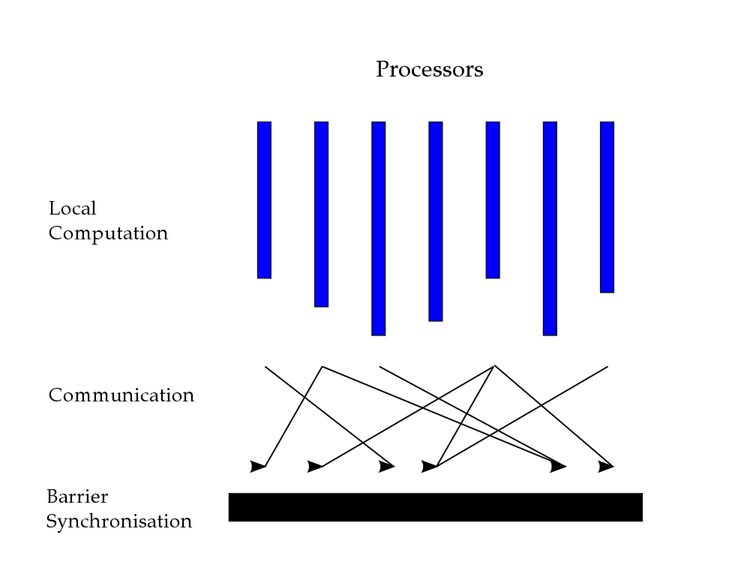
Indeed the OLAP execution mode is very similar in its concept to a Hadoop job (if you are familiar with Hadoop eco-system). In the above picture, we can see that there is a need to synchronize in bulk the different jobs executed on different machines to move from one stage of your traversal to another. This bulk-synchronization is similar to a reduce-step in Hadoop where all the data from different workers are merged together .

Because of the differences in execution model, users of Gremlin OLAP should pay attention to the following points:

A. sideEffect scope

Since in OLAP mode the computation is distributed among different machines, you may not be able to have a global view of the side effect until a synchronization barrier is reached.

Let’s consider the following traversal:

gremlin>g.V().
has("user", "userId", "u861").as("user")                 // Iterator
outE("rated").filter(values("rating").is(gte(9))).inV(). // Iterator
out("belongsTo").values("name").as("genres").            // Save all the genres of well rated movies by this user
...

Because the traversal steps are executed locally on different machine, each machine may label different genres and the genres found on one machine may not be comprehensive. Consequently if you want to re-used the genres label and be sure it contains all the gathered genres, you have to force a synchronization barrier by calling barrier() before accessing the genres label.

B. Path information

With OLAP mode, since all the paths are explored at each stage, we face quickly the combinatorial explosion and thus keeping and processing path information is very expensive and is not practical since it requires sending path information data between machines involved in the computation of the traversal

C. Global ordering

Because Gremlin OLAP is using a Map/Reduce approach, mid-traversal global ordering is useless and is a waste of resource. For example:

gremlin>g.V().
   hasLabel("user"). // Step 1
   order().by("age", decr). // Step 2
   out("rated").values("title") // Step 3

At step 2, we perform a global ordering of all users by their age. It requires a bulk synchronization to gather all user data in a single machine to perform the global ordering, fair enough. But at step 3 (out("rated")), since we continue the traversal, all the ordered user data are again re-broadcasted to multiple machines on the cluster for computation so we will loose the global ordering we just computed.

The only meaningful global ordering in OLAP mode is when it is the last step in the traversal.

IV Note on barriers

All Gremlin steps can be sorted in one of the following categories:

• map: map(), flatMap()…: transform a stream of data type into another data type
• filter: filter(), where(): prune non matching traversers
• sideEffect: store(), aggregate …: perform side effects on the current step and pass the traverser to the next step unchanged
• terminal: next(), toList()…: materialize the lazy evaluation of the traversal into concrete results
• branching: repeat(), choose()…: split the traverser to multiple paths
• collecting barrier: order(), barrier()…: all of the traversers prior to the barrier are collected and then processed before passing to the next step
• reducing barrier: count(), sum()..: all the traversers prior to the barrier are processed by a reduce function and a single reduced value traverser is passed to the next step

That being said, when using Gremlin OLTP you should understand that reaching a barrier step will disable the lazy evaluation nature of your traversal. The traversers are blocked at this barrier until all of them are completely processed before moving to the next step.

V Practical considerations

On the practical side, when you are using Gremlin OLTP you should be aware of some classical caveats:

A. Traversal starting points

Usually for real-time graph exploration people start with an identified vertex (e.g. access vertex by id or with some indices) or a very limited set of vertices and then expand from there. Examples

OLTP Pattern from single vertex

gremlin>g.V().
has("user", "userId", "u861").            // Single user
out("rated").                             // All movies he rated
...

gremlin>g.V(). has("user", "userId", "u861"). // Single user out("rated"). // All movies he rated ...

gremlin>g.V().
   hasLabel("user").
   has("age",30).
   has("gender","M").
   has("city","Austin").
   out("rated").
   ...

By limited set of vertices, we mean a handful of vertices, not more than 100 by rule of thumb otherwise you’ll face combinatorial explosion very quickly!

Now an example of OLAP traversal

OLAP Pattern

gremlin>g.V().
   hasLabel("user").                              // Iterator
   order().by(outE("knows").count(),decr).        // Global ordering on ALL users
limit(1)                                          // Take the 1st in the list  
...

B. Combinatorial explosion

Even if you manage to reduce the number of vertices as your traversal starting point, things can go quickly out of control pretty fast. Indeed, every time you navigate through an edge, it involves an 1-to-N relationship, with N being arbitrary large. In worst case, where your vertex is a super node, the number of adjacent edges can be millions!

So let’s take the previous OLTP example:

OLPT Pattern from Single Vertex

gremlin>g.V().
   has("user", "userId", "u861").                 // Single user
   out("knows").                                  // All users he knows
...

How can you be sure that user u861 has a limited/reasonable number of outgoing knows edges ??? It can range from 0/1 to 10 000. If you don’t know your dataset prior to the traversal, there can be some safeguards:

• count the adjacent edges cardinality for a given vertex
• limit the expansion with sampling
• limit the expansion with selective filtering

Counting edge Cardinality

gremlin>g.V().
   has("user", "userId", "u861").          // Single user
   outE("knows").count()                   //
...

Limiting Exapnision with Sampling

gremlin>g.V().
   has("user", "userId", "u861").          // Single user
   out("knows").sample(100)                // Take maximum 100 friends
...

sample() is a convenient step to limit graph rapid explosion but it has a serious drawback that with sampling you loose any exhaustivity in your traversal. That’s the price to pay to limit resources usage.

Another strategy is to use very restrictive filtering to avoid explosion:

Limiting Expansion with Sampling

gremlin>g.V().
   has("user", "userId", "u861"). // Single user
   out("knows").
   has("age",30).
   has("gender","M")
   ...

Though, filtering is not a silver bullet since it require creating relevant indices before hand and even with filtering, if you don’t know the distribution of your dataset, you don’t know indeed how restrictive your filters are so with the above traversal with restriction on age and gender, we may end with millions of friends !!!

As we can see, without extreme care, any Gremlin OLTP traversal can turn quickly into a full scan/OLAP workload. This is the major trap for beginners.

And that’s all folks! This is the last Gremlin recipe. I hope you had fun following this series..

If you have any question about Gremlin, find me on the datastaxacademy.slack.com, channel dse-graph. My id is @doanduyhai