

Blueprints was not feeling well… He wheeled himself into Apache TinkerPop™ Medical Center for treatment. Upon entering the world class facility, Rexster, the emergency room clerk, brought Blueprints a personal information request form affixed to a clipboard. The form required the following patient information be answered:
- Are you familiar with your graph’s growth characteristics?
- Do you typically run OLTP or OLAP traversals over your graph?
- Do your traversals require path history to be recorded?
After filling out his medical history and sitting through a deliriously long forty minute wait, Furnurse finally approached and greeted the now pale blue Blueprints. Blueprints was escorted to a private screening area for further examination.
- “Hēllõ Mr. Prïñts. Höw bád bàd yôù fèél tôdåÿ?”
- “Well madam..? [in a proper British accent] I must say that I am a bit under the weather. My vim and vigor has lost me these last few days and I’m hoping you and your fine medical staff will be able to rid me of my unfortunate state of affairs.”
- “Yęs.”
- “‘Yes’, what?”
- “Døktör Grėmlîñ cœm sōōń. Nòw nów, Furnurse täkë vįtåls.”
- “Excellent. While I tried to answer the medical request form as a faithfully as possible, there are some items I was just not sure about.”
This article will present analogies between medical and graphical diagnoses and treatments. In both fields, it is important to leverage patient symptoms and vitals in determining the nature of the individual’s affliction/disease. With an accurate diagnoses, any number of treatments can be applied to the illness with the end goal of creating a happy, healthy, flourishing being — human or graph system.
Graph Vitals: Graph → Number(s)

Vitals are an important aspect of any medical diagnoses because they distill the complexities of a person into a set of descriptive (and ultimately prescriptive) numbers. They can be defined as functions that map a person to a value. For instance, age: P → ℕ+ — marko ∈ P, age(marko) → 29. Other example human vitals include: heart rate, blood pressure, age, weight, and height. Their function signatures are provided which define the function name (xyz:) and its domain P (the set of all people) and range, where ℕ is the set of natural numbers (int), ℝ is the set of real numbers (float), and × is the cross product of two sets (e.g. pair<int>).
heartRate: P → ℕ+ |
Maps a person to a positive integer. |
bloodPressure: P → ℕ+ × ℕ+ |
Maps a person to a pair of positive integers (i.e. systolic and diastolic pressure). |
weight: P → ℝ+ |
Maps a person to a positive real number (e.g. kilograms). |
height: P → ℝ+ |
Maps a person to a positive real number (e.g. meters). |
| Graph Obstetrics | |||
|---|---|---|---|
|
|
|||
 |
|||
 |
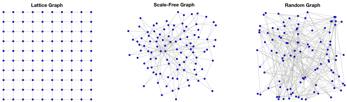
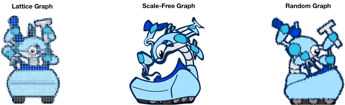
The first graph is a lattice graph. Lattices are formed when a single graph motif is repeated in every direction along the dimensions of the lattice’s embedding. Geologically, lattices typically emerge in highly controlled environments under intense pressure/heat such as in the case of the morphing of a carbon source into diamond. Many top-down human endeavors create lattices. Power grids, road networks, and management hierarchies are all examples of manmade lattice-like graphs. |
||
| This panel has been intentionally left blank. |  |
The second graph is a scale-free graph. Scale-free graphs are predominate across numerous natural systems. There are many algorithms to create scale-free networks, but perhaps the simplest and easiest to understand is preferential attachment, where a newly introduced vertex is more likely to attach to an already existing vertex with many edges than to a vertex that has few edges. This growth pattern is colloquially known as “the rich get richer.” Scale-free graphs have few vertices with a high degree and many vertices with a low degree. For instance, most people on Twitter have few followers ( |
|
|
Finally, a random graph is one where the number of edges any one vertex has is determined by a Gaussian (or normal) distribution. The growth algorithm for random graphs is simple. A set of vertices is created. Then, when an edge is added, two vertices are selected at random and connected. Unlike preferential attachment, in random graph construction, there is no bias when selecting which vertices to connect. Contrary to popular thought, and unlike scale-free graphs and lattices, random graphs typically do not appear in nature and have only served the domain of graph theory as a purely theoretical structure for which theorems are easily proved on. |
|||
 Blueprints isn’t a human and therefore vitals such as blood pressure, age, weight, and height don’t apply. Instead, the vitals for a graph include: vertex count, edge count, and degree distribution.
vertexCount: G → ℕ+ |
Maps a graph to a positive integer. |
edgeCount: G → ℕ+ |
Maps a graph to a positive integer. |
degreeDistribution: G → ℘(ℕ+ × ℕ+) |
Maps a graph to a set of integer pairs (i.e. Map<Integer,Integer>). |
- “Furnurse cøûnt hòw mänÿ vértīcès âńd èdgés hävę ÿöü. Thėn Furnurse dō fûll scân ôf yøūr vèrtéx sêt tö crèátê dègrēé dįstrįbūtįōñ.”
- “Excellent, this is exactly the specifics I was unable to answer in your patient information request form.”
- “Ÿės.”
- “‘Yes’, what?!”
- “Økáÿ.”
Basic graph statistics such as vertex count, edge count, and degree distribution require a full scan of the entire graph. Such global analyses can be evaluated in a parallel manner more efficiently and are typically calculated using an OLAP/analytics execution engine like GraphComputer on the Gremlin traversal machine. While counting vertices and edges are straightforward, creating a degree distribution is a bit more involved. In the analysis below, there is 1 vertex that has a degree of 16, 55 vertices with a degree of 2, so forth and so on. The vertex and edge counts for all three example graphs are provided in the table below.
gremlin> g.V().count()==>100gremlin> g.E().count()==>197gremlin> g.V().groupCount().by(both().count())==>[16:1,2:55,3:16,4:6,5:5,6:4,7:3,8:2,9:5,10:1,27:1,28:1] |
| Lattice Graph | Scale-Free Graph | Random Graph | |
g.V().count() |
100 | 100 | 100 |
g.E().count() |
180 | 197 | 198 |
Furnurse gathered the requisite vitals from Blueprints and left the private screening room. After an excruciatingly long 45 minute wait, Dr. Gremlin moseyed into the Blueprints’ examination room.
- “How are you doing there Mr. Prints?”
- “I’m doing the same thing I was doing before I came to the hospital — waiting for processes to complete!”
- “Yes, well, in these topsy turvy times…”
- “In these ‘topsy turvy times’ what?”
- “So after looking over your vitals, I note that you don’t have a large graph and thats good. However, if traversal complexity was simply a function of vertex and edge counts, well, I wouldn’t have to go 4 years of ‘Maniacal Doctor School’ to diagnose your problem. What is troubling me about your vital statistics has to do primarily with your degree distribution. If you look closely at the plot Furnurse generated for us, there are numerous vertices in your graph with a low degree while only a few have a high degree?”
- “Yes, I see that. I believe that is because every time I add a vertex to my graph, I am more likely to connect it to an already existing popular vertex.”
- “Ah, yes — the old cumulative advantage bias leads to a graph model (or phenotype) known as scale-free. Don’t be alarmed, this is a very natural growth. However, scale-free graphs, while typical of real-world system modeling, can lead to unexpected traversal behavior.
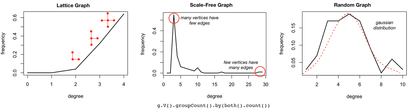
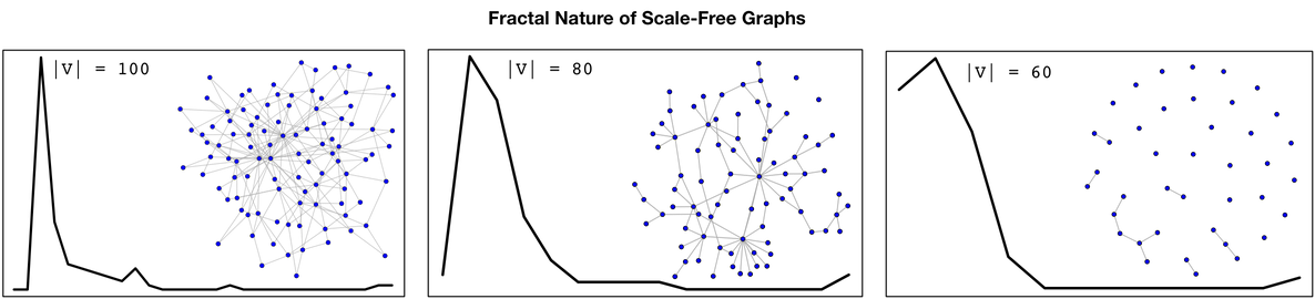
The space of abstract graph models can be generally understood as being on a spectrum from highly organized (lattice graphs) to highly disorganized (random graphs). Two dimensional lattices have three graph motifs: corner vertices, border vertices, and internal vertices with the internal vertices forming the bulk of the lattice’s structure. This consistency of form ensures predictable traversal performance. Random graphs on the other hand do not have any repeatable/compressible/patterned internal structure. The lack of bias when connecting two vertices leads to a degree distribution where all vertices have the same degree (save some outliers on either side of the mean). While random graphs are randomly created, they actually have predictable traversal performance because all vertices are nearly identical in that their degree is centered around a shared mean. In between lattices and random graphs are scale-free graphs. These graphs have a more complex repeating motif, yet a motif nonetheless. The motif is a “super vertex” (a high degree vertex) and numerous adjacent “satellite vertices” (low degree vertices) along with their respective connections. As demonstrated in the diagram below, this pattern is repeated in a fractal manner, where in any extracted subgraph of the full scale-free graph, there are always, relatively speaking, few high degree vertices and very many low degree vertices.
The degree distributions of these abstract graph models are distinct and easy to compute. It is for this reason that degree distribution should be derived throughout the evolution of a graph system in order to understand the graph’s global connectivity pattern and its effect on traversal performance.
Graph Diagnosis: Number(s) → Problem
In some situations, basic statistics (or vitals) on a system are sufficient to yield a diagnoses. In general, a diagnoses is abstractly defined as a function that takes an ordered pair of symptoms and vitals and maps it to a known, categorical illness.
diagnosis: ℘(Symptom) × ℘(Vital) → Illness
For instance, if a person is extremely thirsty and weighs 135 kilograms, then a potential diagnoses is diabetes. However, if that person is 85 meters in height, then the diagnoses may simply be dehydration. Thus, weight alone is not a good predictor of someone’s obesity and thus, a predictor of the root cause of their thirst. For this reason, there exists composite statistics such as body mass index, where bmi: weight(P) × height(P) → ℝ+. Now, if the thirsty individual has a large BMI, then diabetes may certainly be the associated illness.
- “I have a very low vertex and edge count. Why would my system be under stress?”
- “Yes, when analyzed alone, your vertex and edge counts look good. However, when comparing the edge counts of each vertex, a more telling picture emerges. Your degree distribution and your growth algorithm are a sure sign of a scale-free structure. Again, scale-free graphs are perfectly natural, its just that they can have numerous paths through them compared to other types of graphs with the same vertex and edge counts.
- “Is it bad to have numerous paths?”
- “No not at all. In fact, this is one of the most touted features of scale-free graphs. Random attacks on such graphs have a difficult time isolating any two vertices from each other. It is difficult to take a strongly connected scale-free graph and partition it. In other words, scale-free graphs are extremely robust structures. This is perhaps why nature tends towards them. However, the problems that emerge with such graphs tend to be on the processing side of things — with durable connectivity, comes many paths. Do you mind telling me what type of traversals you are running these days?”
- “I dunno — simple queries.”
- “And what does ‘simple’ mean to you?”
- “Acyclic path walks.”
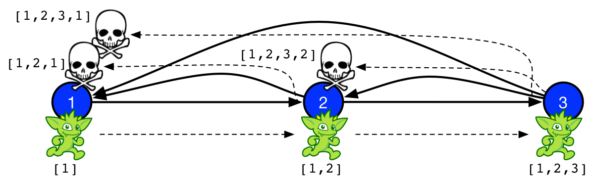
- “Well, that might be exactly why you feel so tired. Graphs with large path counts and traversals with path history do not mix well. Let me explain — if you need to know if a particular traverser has already been to a previous vertex along its walk, then it needs to remember/save/index the past vertices it has touched. Keeping all that information around is memory intensive, but also, it reduces the likelihood that any two traversers will be able to be ‘bulked’ (i.e. merged into a single traverser).”
Dr. Gremlin decided to run one more analysis to show Blueprints the nature of his problem. The problem was not so much his structure, nor as will be shown later, the process. Instead, the problem existed at the intersection of both structure (graph) and process (traversal).
gremlin> clockWithResult(10){ g.V().repeat(both().simplePath()).times(1).count().next() }==>0.35125999999999996==>394gremlin> clockWithResult(10){ g.V().repeat(both().simplePath()).times(2).count().next() }==>1.225206==>2884gremlin> clockWithResult(10){ g.V().repeat(both().simplePath()).times(3).count().next() }==>6.3554569999999995==>16056gremlin> clockWithResult(10){ g.V().repeat(both().simplePath()).times(4).count().next() }==>37.253097==>79346gremlin> clockWithResult(10){ g.V().repeat(both().simplePath()).times(5).count().next() }==>184.311016==>357836gremlin> clockWithResult(10){ g.V().repeat(both().simplePath()).times(6).count().next() }==>889.4046159999999==>1469578gremlin> clockWithResult(10){ g.V().repeat(both().simplePath()).times(7).count().next() }==>3797.08549==>5528946gremlin> clockWithResult(10){ g.V().repeat(both().simplePath()).times(8).count().next() }==>15003.055819==>19362114gremlin> clockWithResult(10){ g.V().repeat(both().simplePath()).times(9).count().next() }==>57232.158837999996==>63910882gremlin> clockWithResult(10){ g.V().repeat(both().simplePath()).times(10).count().next() }==>192643.540888==>200146166 |
Graph Treatment: Problem → Solution
When a medical problem is identified. The solution (e.g. a drug) is prescribed. For common ailments, doctors will use a medical reference book (i.e. HashMap<Illness,Set<Cure>>) to identify the cure to the diagnosed disease. Such reference manuals may have multiple cures for the same illness (℘(Cure)) — each with their respective benefits and drawbacks.
treatment: Illness → ℘(Cure)
- “There are basically only two ways to solve your problem. We can either 1.) alter your graph structure to reduce path count or we can 2.) alter your traversal process to reduce traverser count.”
- “I don’t quite understand the distinction. Can you go over my options more clearly?”
- “Yes, definitely. First, let’s look at changing your structure and leaving your acyclic traversal as is. We can make your graph structure either more lattice-like or more random-like. Looking at the table and plots provided by Furnurse, you can see that your scale-free nature yields way more simple paths than either the lattice- or random-graph structures — even though vertex and edge counts are the virtually the same! It is ultimately this path growth which is causing you to feel rundown and out of energy. Your traversal is simply examining too many paths and this, in turn, is exhausting your computing resources.”
g.V().repeat(both().simplePath()).times(x).count()
| Lattice Graph | Scale-Free Graph | Random Graph | ||||
| path length | path count | time (ms) | path count | time (ms) | path count | time (ms) |
g.V().repeat(both().simplePath()).times(x).count() |
||||||
| 1 | 360 | 0.307 | 394 | 0.351 | 396 | 0.219 |
| 2 | 968 | 0.584 | 2884 | 1.225 | 1610 | 0.794 |
| 3 | 2656 | 2.018 | 16056 | 6.336 | 6420 | 3.644 |
| 4 | 6672 | 5.284 | 79346 | 37.253 | 24820 | 13.456 |
| 5 | 17272 | 14.962 | 357836 | 184.311 | 94342 | 55.246 |
| 6 | 42832 | 38.269 | 1469578 | 889.404 | 353296 | 223.498 |
| 7 | 108296 | 107.371 | 5528946 | 3797.085 | 1299046 | 901.398 |
| 8 | 265280 | 291.853 | 19362114 | 15003.056 | 4698148 | 3556.033 |
| 9 | 657848 | 744.061 | 63910882 | 57232.158 | 16698554 | 13657.287 |
| 10 | 1593024 | 1964.040 | 200146166 | 192643.540 | 58335788 | 51064.125 |
The simplePath()-step filters out traversers whose path history contains repeats. For every step in the traversal (times(x)), the number of simple paths in a lattice graph more than doubles. For a random graph, it more than triples. For a scale-free graph, it more than quadruples. It is this growth rate which yields the respective increase in time because when using path-based steps like simplePath(), each traverser is required to remember its path history and thus, each traverser must be uniquely identified in the computation. Thus, the more paths, the more traversers. The more traversers, the more processing required to execute the traversal. It is this simple dependency that binds path count to traversal execution time in a near 1-to-1 relationship when path history is required.
| Lattice Graph | Scale-Free Graph | Random Graph | |
| path growth rate | 2.385 | 4.460 | 3.756 |
| time growth rate | 2.675 | 4.412 | 3.957 |
- “If you like your scale-free graph structure the way it is, then you can change your traversal process. Have you considered not worrying about filtering out cyclic paths? If you simply remove
simplePath()-step from your traversal, then your traversers will not be required to remember their history. The benefit of this is that when a traverser no longer has to remember its past, its present state is its only defining characteristic and an optimization known as ‘bulking’ is more likely.
g.V().repeat(both()).times(x).count()
| Lattice Graph | Scale-Free Graph | Random Graph | ||||
| path length | path count | time (ms) | path count | time (ms) | path count | time (ms) |
g.V().repeat(both()).times(x).count() |
||||||
| 1 | 360 | 0.232 | 394 | 0.172 | 396 | 0.235 |
| 2 | 1328 | 0.288 | 3278 | 0.243 | 2006 | 0.361 |
| 3 | 4952 | 0.356 | 22404 | 0.423 | 10096 | 0.453 |
| 4 | 18592 | 0.437 | 176002 | 0.412 | 51986 | 0.448 |
| 5 | 70120 | 0.637 | 1294686 | 0.508 | 267054 | 0.546 |
| 6 | 265352 | 0.712 | 10010512 | 0.534 | 1379704 | 0.551 |
| 7 | 1006704 | 0.713 | 75100132 | 0.609 | 7118188 | 0.654 |
| 8 | 3826976 | 0.737 | 575885466 | 0.679 | 36804834 | 0.723 |
| 9 | 14571464 | 0.844 | 4352964178 | 0.856 | 190135196 | 0.787 |
| 10 | 55554808 | 1.010 | 33239692938 | 1.026 | 983296372 | 0.896 |
By removing the simplePath()-step, traversers no longer have to keep track of their path history. Their only state is their location in the graph (data) and their location in the traversal (program). These memory-less traversers can be subjected to something called bulking in the Gremlin traversal machine. If two traversers are at the same vertex and same step, then they can be merged into a single traverser with a bulk of 2. Likewise, if two traversers each with bulk 5 and 10 meet at the same locations, then a single traverser can be created with bulk of 15. Next, instead of executing the next step/instruction 15 times (once for each traverser), it is possible to only execute it only once and set the bulk of the resultant traverser to 15. The end effect is that the path count is no longer correlated with the execution time. Bulking is a graph processing compression technique that reduces space and leverages computational memoization to reduce time.
| Lattice Graph | Scale-Free Graph | Random Graph | |
| path growth rate | 3.771 | 7.607 | 5.135 |
| time growth rate | 1.184 | 1.236 | 1.169 |
- “Yes. Lets go with altering my traversal and avoid the space/time costs associated with
simplePath().” - “Very well, off to surgery we go!”
Conclusion
Computing can be understood as the interplay of a data structure and an algorithmic process. As such, the complexity of any computing act can be altered by either changing the data structure or changing the algorithmic process. The purpose of this article was to demonstrate that different graph models can yield wildly different performance characteristics for the same traversal — even when the graphs have the same number of vertices and the same number of edges. However, because graphs are interconnected structures, count-based statistics are typically not sufficient as the only means of predicting the performance of a traversal. More structural statistics such as degree distribution will provide greater insight into the general connectivity patterns of the graph. These connectivity patterns (or graph models) are much better predictors of traversal performance.
In practice, it is usually not possible to alter the graph structure as the structure is a function of a real-world system being modeled. While there are modeling optimizations that can be accomplished to alter general connectivity patterns, most of the performance gains will come from changing the traversal process. In particular, traversals that don’t make use of side-effect data such as path histories should be avoided if possible. On the Gremlin graph traversal machine, this means avoiding steps such as those itemized in the table below. Note that requiring full path data is much more costly and much less likely to yield bulked traversers than the labeled path traverser requirement. Labeled paths only record those path segments that have been labeled with as() and moreover, once the labeled path section is no longer required, it can be dropped mid-traversal. This has the benefit of reducing the memory footprint and increasing the likelihood of subsequent bulking (see PathRetractionStrategy).
| Step | Traverser Requirement | Description |
path() |
full path | Maps a traverser to its path history. |
simplePath() |
full path | Filters a traverser that has cycles in its path history. |
cyclicPath() |
full path | Filters a traverser that does not have cycles in its path history. |
tree() |
full path | Maps all traversers (via a barrier) to an aggregate tree data structure. |
select() |
labeled path | Maps a traverser to a previously seen object in its path. |
where() |
labeled path | Filters a traverser based on a previously seen object in its path. |
match() |
labeled path | Maps a traverser to a particular set of bindings in its path history. |
The information presented herein provides the graph user the tools they need to help diagnose potential performance issues in their graph application. By understanding the relationship between structure and process, the user will be more fit to immediately recognize potential problems in either how their graph is growing or how their traversals are being written.
- “Ï háppÿ ÿøū fèél bęttėr, Mr. Prïnts.”
- “Thank you Furnurse. Your team has done an outstanding job diagnosing my problem and going over my treatment options. I feel great now that I’m running a memory-less traversal. Once again I’m full of vim and vigor!”
- “Ÿės.”
More Technology
View All
How to Create a Local LangChain Vector Database

Apache Cassandra 2024 Wrapped: A Year of Innovation and Growth

How We Built UnReel: An AI-Generated, Multiplayer Movie Quiz